15 Analysis of variance

15.1 Introduction

This chapter is about an often used statistical analysis, called analysis of variance (often abbreviated to ANOVA).

The structure of this chapter is as follows. We will begin in §15.2 with some examples of research studies whose outcomes can be tested with analysis of variance. The purpose of this section is to familiarise you with the technique, with the new terminology, and with the conditions under which this technique can be used. In §15.3.1, we will introduce this technique in an intuitive manner by looking at the thinking behind the test. In §15.3.2 we derive a formal form for the most important test statistic, the \(F\)-ratio.

15.2 Some examples

Just like the t-test, analysis of variance is a statistical generalisation technique, which is to say: an instrument that can be used when formulating statements about the population characteristics, on the basis of data taken from samples from these populations. In the case of the t-test and ANOVA, the statements are about whether or not the means of (two or more) populations are equal. In this sense, analysis of variance can also be understood as an expanded version of the t-test: we can analyse data of more than two samples with ANOVA. Moreover, it is possible to include the effects of multiple independent variables simultaneously in the analysis. This is useful when we want to analyse data from a factorial design (§6.8).

Examples 15.1: In this example, we investigate the speech tempo or speed of four groups of speakers, namely originating from the Middle, North, South and West of the Netherlands. The speech tempo is expressed as the mean duration of a syllable (in seconds), with the mean taken over an interview of approximately 15 minutes with each speaker (Quené 2008) (R-hqmisc?). A shorter mean syllable duration thus corresponds to a faster speaker (cf. skating, where a faster skater has shorter lap durations). There were 20 speakers per group, but 1 speaker (from the South), who had an extremely high value, was removed from the sample.

The observed speech tempos per speaker from the above Example 15.1 are summarised in Table 15.1 and Figure 15.1.

Here, the region of origin is an independent categorial variable or ‘factor’. The values of this factor are also referred to as ‘levels’, or in many studies as ‘groups’ or ‘conditions’. Each level or each group or condition forms a ‘cell’ of the design, and the observations from that cell are also called ‘replications’ (consider why they are called this). The speech tempo is the dependent variable. The null hypothesis is that the dependent variable means are equal for all groups, thus H0: \(\mu_M = \mu_N = \mu_Z = \mu_W\). If we reject H0, then that means only that not all means are equal, but it does not mean that each group mean deviates from each other group mean. For this, a further (post-hoc) study is necessary; we will return to this later.

Table 15.1: Mean speech tempos, with standard deviation and numbers of speakers, divided according to region of origin of the speaker (see Example 15.1).
Region	Mean	s.d.	n
Middle	0.253	0.028	20
North	0.269	0.029	20
South	0.260	0.030	19
West	0.235	0.028	20

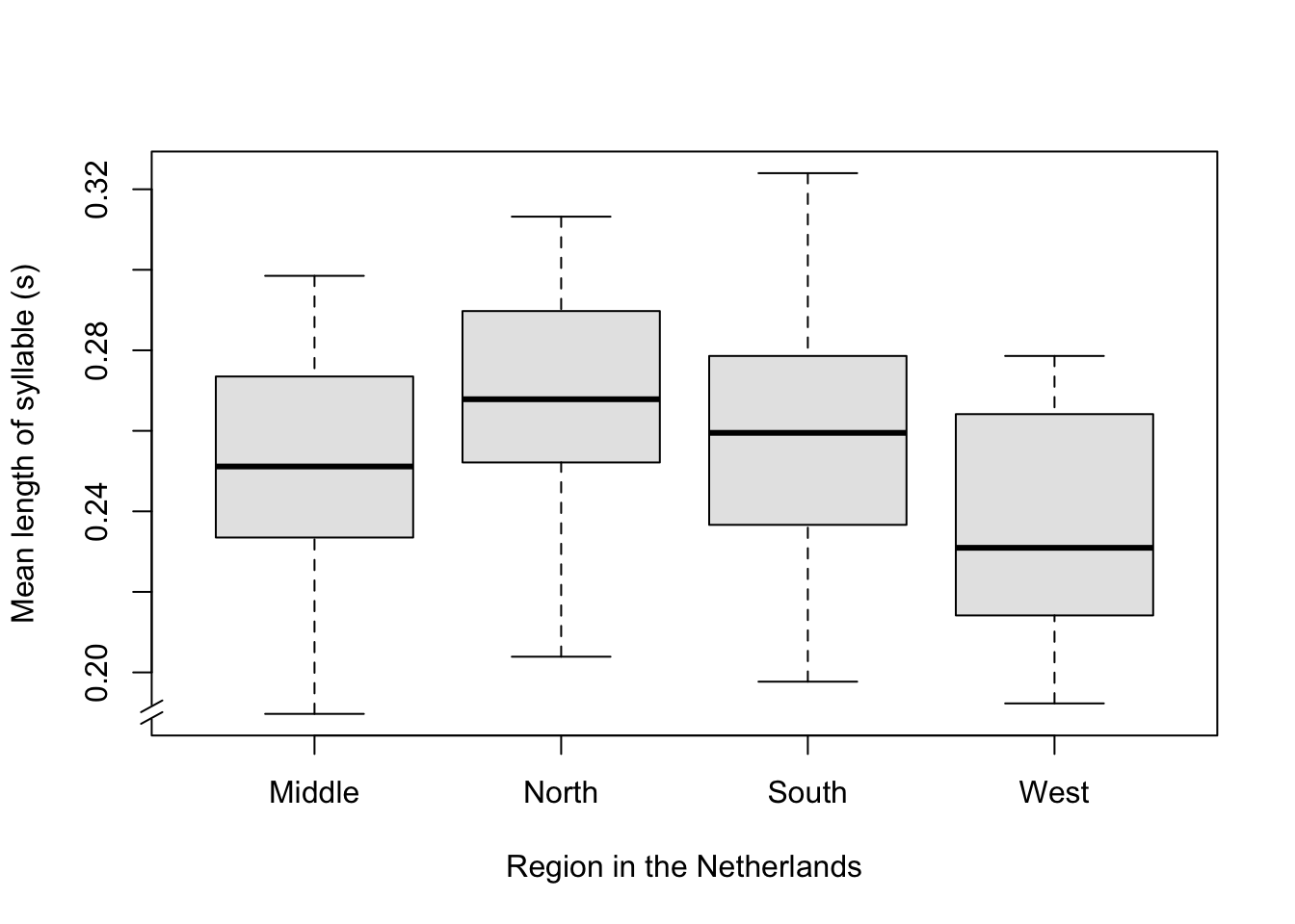
Figure 15.1: Boxplot of the mean length of syllable, split up according to region of origin of the speaker.

In order to investigate whether the four populations differ in their average speech tempo, we might think about conducting t-tests for all pairs of levels. (With 4 levels, that would require 6 tests, see equation (10.6) with \(n=4\) and \(x=2\)). There are however various objections to this approach. We will discuss one of these here. For each test, we use a p-value of \(\alpha=.05\). We thus have a probability of .95 of a correct decision without a Type I error. The probability that we will make a correct decision for all 6 tests is \(.95^6 = .731\) (according to the multiplication principle, equation (10.4)). The joint probability of one or more Type I error(s) in the 6 tests is thus no longer \(.05\), but has now increased to \(1-.731 = .265\), more than a quarter!

Analysis of variance now offers the possibility of investigating the aforementioned null hypothesis on the basis of a single testing (thus not 6 tests). Analysis of variance can thus be best characterised as a global testing technique, which is most suitable if a priori you are not able or do not want to make any specific predictions about the differences between the populations.

An analysis of variance applied to the scores summarised in Table 15.1 will lead to the rejection of the null hypothesis: the 4 regional means are not equal. The differences found are, in all probability, not due to chance sample fluctuations, but instead to systematic differences between the groups (\(\alpha=.05\)). Can it now be concluded that the differences found in speech tempo are caused by differences in the origin of the speaker? Here, restraint is required (see §5.2). After all, it cannot be excluded that the four populations not only differ systematically from each other in speech tempo, but also in other relevant factors which were not included in the study, such as health, wealth, or education. We would only be able to exclude these other factors if we allocated the participants randomly to the selected levels of the independent variable. However, this is not possible when we are concerned with the region of origin of the speaker: we can usually assign a speaker (randomly) to a form of treatment or condition, but not to a region of origin. In fact, the study in Example 15.1 is thus quasi-experimental.

For our second example, we involve a second factor in the same study on speech tempo, namely also the speaker’s gender. ANOVA enables us, in one single analysis, to test whether (i) the four regions differ from each other (H0: \(\mu_M = \mu_N = \mu_Z = \mu_W\)), and (ii) whether the two genders differ from each other (H0: \(\mu_\textrm{woman} = \mu_\textrm{man}\)), and (iii) whether the differences between the regions are the same for both genders (or, put differently, whether the differences between the genders are the same for all regions). We call the latter differences the ‘interaction’ between the two factors.

Table 15.2: Mean speech tempos, with standard deviation and numbers of speakers, divided according to gender and the speaker’s region of origin (see Example 15.1).
Gender	Region	Mean	s.d.	n
Woman	Middle	0.271	0.021	10
Woman	North	0.285	0.025	10
Woman	South	0.269	0.028	9
Woman	West	0.238	0.028	10
Man	Middle	0.235	0.022	10
Man	North	0.253	0.025	10
Man	South	0.252	0.030	10
Man	West	0.232	0.028	10

The results in Table 15.2 suggest that (i) speakers from the West speak more quickly than the others, and that (ii) men speak more quickly than women (!). And (iii) the difference between men and women appears to be smaller for speakers from the West than for speakers from other regions.

15.2.1 assumptions

The analysis of variance requires four assumptions which must be satisfied to use this test; these assumptions match those of the t-test (§13.2.3).

The data have to be measured on an interval level of measurement (see §4.4).
All observations have to be independent of each other.
The scores have to be normally distributed within each group (see §10.4).
The variance of the scores has to be (approximately) equal in the scores of the respective groups or conditions (see §9.5.1). The more the samples differ in size, the more serious violating this assumption is. It is thus sensible to work with equally large, and preferably not too small samples.

Summarising: analysis of variance can be used to compare multiple population means, and to determine the effects of multiple factors and combinations of factors (interactions). Analysis of variance does require that data satisfy multiple conditions.

15.3 One-way analysis of variance

15.3.1 An intuitive explanation

As stated, we use analysis of variance to investigate whether the scores of different groups, or those collected under different conditions, differ from each other. However — scores always differ from each other, through chance fluctuations between the replications within each sample. In the preceding chapters, we already encountered many examples of chance fluctuations within the same sample and within the same condition. The question then is whether the scores between the different groups (or gathered under different conditions) differ more from each other than you would expect on the basis of chance fluctuations within each group or cell.

The aforementioned “differences between scores” taken together form the variance of those scores (§9.5.1). For analysis of variance, we divide the total variance into two parts: firstly, the variance caused by (systematic) differences between groups, and secondly, the variance caused by (chance) differences within groups. If H0 is true, and if there are thus no differences (in the populations) between the groups, then we nevertheless expect (in the samples of the groups) some differences between the mean scores of the groups, be it that the last mentioned differences will not be greater than the chance differences within the groups, if H0 is true. Read this paragraph again carefully.

This approach is illustrated in Figure 15.2, in which the scores from three experimental groups (with random assignment of participants to the groups) are shown: the red, grey and blue group. The scores differ from each other, at least through chance fluctuations of the scores within each group. There are probably also systematic differences between (the mean scores of) the three groups. However, are these systematic differences now comparatively larger than the chance differences within each group? If so, then we reject H0.

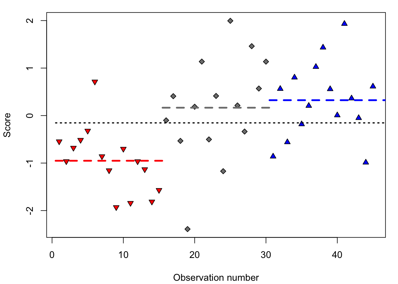
Simulated observations of three experimental groups: red (downwards triangle), grey (diamond), and blue (upwards triangle) (n=15 per group), with the mean per group (in dashed lines), and with the mean over all observations (dotted line).

Figure 15.2: Simulated observations of three experimental groups: red (downwards triangle), grey (diamond), and blue (upwards triangle) (n=15 per group), with the mean per group (in dashed lines), and with the mean over all observations (dotted line).

The systematic differences between the groups correspond with the differences from the red, grey and blue group means (dashed lines in Figure 15.2) relative to the mean over all observations (dotted line). For the first observation, that is a negative deviation since the score is below the general mean (dotted line). The chance differences within the groups correspond to the deviation of each observation relative to the group mean (for the first observation that is thus a positive deviation, since the score is above the group average of the red group).

Let us now make the switch from ‘differences’ to ‘variance’. We then split the deviation of each observation relative to the general mean into to two deviations: first, the deviation of the group mean relative the general mean, and, second, the deviation of each replication relative to the group mean. These are two pieces of variance which together form the total variance. Vice versa, we can thus divide the total variance into two components, which is where the name ‘analysis of variance’ comes from. (In the next section, we will explain how these components are calculated, taking into account the number of observations and the number of groups.)

Dividing the total variance into two variance components is useful because we can determine the ratio between these two parts. The ratio between the variances is called the \(F\)-ratio, and we use this ratio to test H0.

\[\textrm{H0}: \textrm{variance between groups} = \textrm{variance within groups}\]

\[\textrm{H0}: F = \frac{\textrm{variance between groups}}{\textrm{variance within groups}} = 1\]

As such, the \(F\)-ratio is a test statistic whose probability distribution is known if H0 is true. In the example of Figure 15.2, we find \(F=3.22\), with 3 groups and 45 observations, \(p=.0004\). We thus find a relatively large systematic variance between groups here, compared to the relatively small chance variance within groups: the former variance (the fraction \(F\)’s numerator) is more than \(3\times\) as large as the latter variance (the fraction \(F\)’s denominator). The probability \(p\) of finding this fraction if H0 is true, is exceptionally small, and we thus reject H0. (In the following section, we will explain how this probability is determined, again taking into account the number of observations and the number of groups.) We then speak of a significant effect of the factor on the dependent variable.

At the end of this section, we repeat the core essence of
analysis of variance. We divide the total variance into two parts: the possible systematic variance between groups or conditions, and the variance within groups or conditions (i.e. ever present, chance fluctuation between replications). The test statistic \(F\) consists of the proportion between these two variances. We do a one-sided test to see whether \(F=1\), and reject H0 if \(F>1\) such that the probability \(P(F|\textrm{H0}) < \alpha\). The mean scores of the groups or conditions are then in all probability not equal. With this, we do not yet know which groups differ from each other - for this another further (post-hoc) analysis is needed (§15.3.5 below).

15.3.2 A formal explanation

For our explanation, we begin with the observed scores. We assume that the scores are constructed according to a certain statistical model, namely as the sum of the population mean (\(\mu\)), a systematic effect (\(\alpha_j\)) of the \(j\)’the condition or group (over \(k\) conditions or groups), and a chance effect (\(e_{ij}\)) for the \(i\)’the replication within the \(j\)’the condition or group (over \(N\) replications in total). In formula: \[x_{ij} = \mu + \alpha_{j} + e_{ij}\] Here too, we thus again analyse each score in a systematic part and a chance part. This is the case not only for the scores themselves, but also for the deviations of each score relative to the total mean (see §15.3.1).

Thus, three variances are of interest. Firstly, the total variance (see equation (9.3), abbreviated to t) over all \(N\) observations from all groups or conditions together: \[\begin{equation} \tag{15.1} s^2_t = \frac{ \sum (x_{ij} - \overline{x})^2 } {N-1} \end{equation}\] Secondly the variance ‘between’ (abbreviated to b) the groups or conditions: \[\begin{equation} \tag{15.2} s^2_b = \frac{ \sum_{j=1}^{j=k} n_j (\overline{x_j} - \overline{x})^2 } {k-1} \end{equation}\] and, thirdly, the variance ‘within’ (shortened to w) the groups or conditions: \[\begin{equation} \tag{15.3} s^2_w = \frac{ \sum_{j=1}^{j=k} \sum_i (x_{ij} - \overline{x_j})^2 } {N-k} \end{equation}\]

In these comparisons, the numerators are formed from the sum of the squared deviations (‘sums of squares’, shortened to SS). In the previous section, we indicated that the deviations add up to each other, and that then is also the case for the summed and squared deviations: \[\begin{align} \tag{15.4} { \sum (x_{ij} - \overline{x})^2 } &= { \sum_{j=1}^{j=k} n_j (\overline{x_j} - \overline{x})^2 } + { \sum_{j=1}^{j=k} \sum_i (x_{ij} - \overline{x_j})^2 } \\ \textrm{SS}_t &= \textrm{SS}_b + \textrm{SS}_w \end{align}\]

The numerators of the variances are formed from the degrees of freedom (abbreviated df, see §13.2.1). For the variance between groups \(s^2_b\), that is the number of groups or conditions, minus 1 (\(k-1\)). For the variance within groups \(s^2_w\), that is the number of observations, minus the number of groups (\(N-k\)). For the total variance, that is the number of observations minus 1 (\(N-1\)). The degrees of freedom of the deviations also add up to each other: \[\begin{align} \tag{15.5} { (N-1) } &= { (k-1) } + { (N-k) } \\ \textrm{df}_t &= \textrm{df}_b + \textrm{df}_w \end{align}\]

The above fractions which describe the variances \(s^2_t\), \(s^2_b\) and \(s^2_w\), are also referred to as the ‘mean squares’ (shortened to MS). \(\textrm{MS}_{t}\) is by definition equal to the ‘normal’ variance \(s^2_x\) (see the identical equations (9.3) and (15.1)).

The test statistic \(F\) is defined as the ratio of the two variance components defined above: \[\begin{equation} \tag{15.6} F = \frac{ s^2_b } { s^2_w } \end{equation}\] with not one but two degrees of freedom, resp. \((k-1)\) for the numerator and \((N-k)\) for the denominator.

You can determine the p-value \(p\) which belongs with the \(F\) found using a table, but we usually conduct an analysis of variance using a computer, and it then also calculates the p-value.

The results of an analysis of variance are summarised in a fixed format in a so-called ANOVA table, like Table 15.3. This contains the most important information summarised. However, the whole table can also be summarised in one sentence, see Example 15.2.

Table 15.3: Summary of analysis of variance of the observations in Figure 15.2.
Variance Source	df	SS	MS	\(F\)	\(p\)
Group	2	14.50	7.248	9.36	<.001
(within)	42	32.54	0.775

Example 15.2: The mean scores are not equal for the red, grey and blue group \([F(2,42) = 9.35\), \(p < .001\), \(\omega^2 = 0.28]\).

15.3.3 Effect size

Just like with the \(t\)-test, it is not only important to make a binary decision about H0, but it is at least equally important to know how large the observed effect is (see also §13.8). This effect size for analysis of variance can be expressed in different measures, of which we will discuss two (this section is based on Kerlinger and Lee (2000); see also Olejnik and Algina (2003)).

The simplest measure is the so-called \(\eta^2\) (“eta squared”), the proportion of the total SS which can be attributed to the differences between the groups or conditions: \[\label{eq:etasq} \eta^2 = \frac{ \textrm{SS}_b } { \textrm{SS}_t }\] The effect size \(\eta^2\) is a proportion between 0 and 1, which indicates how much of the variance in the sample can be assigned to the independent variable.

The second measure for effect size with analysis of variance is the so-called \(\omega^2\) (“omega squared”) (Maxwell and Delaney 2004, 296): \[\begin{equation} \tag{15.7} \omega^2 = \frac{ \textrm{SS}_b - (k-1) \textrm{MS}_w} { \textrm{SS}_t + \textrm{MS}_w } \end{equation}\] The effect size \(\omega^2\) is also a proportion; this is an estimation of the proportion of the variance in the population which can be attributed to the independent variable, where the estimation is of course based on the investigated sample. As we are generally more interested in generalisation to the population than to the sample, we prefer \(\omega^2\) as the measure for the effect size.

We should not only report the \(F\)-ratio, degrees of freedom, and p-values, but also the effect size (see Example 15.2 above).

“It is not enough to report \(F\)-ratios and whether they are statistically significant. We must know how strong relations are. After all, with large enough \(N\)s, \(F\)- and \(t\)-ratios can almost always be statistically significant. While often sobering in their effect, especially when they are low, coefficients of association of independent and dependent variables [i.e., effect size coefficients] are indispensable parts of research results” (Kerlinger and Lee 2000, 327, emphasis added).

15.3.4 Planned comparisons

In Example 15.2 (see Figure 15.2), we investigated the differences between scores from the red, grey and blue groups. The null hypothesis which was tested was H0: \(\mu_\textrm{red} = \mu_\textrm{grey} = \mu_\textrm{blue}\). However, it is also quite possible that a researcher already has certain ideas about the differences between groups, and is looking in a focused manner for certain differences, and wants to actually ignore other differences. The planned comparisons are also called ‘contrasts’.

Let us assume for the same example that the researcher already expects, from previous research, that the red and blue group scores will differ from each other. The H0 above is then no longer interesting to investigate, since we expect in advance that we will reject H0. The researcher now wants to know in a planned way (1) whether the red group scores lower than the other two groups, (H0: \(\mu_\textrm{red} = (\mu_\textrm{grey}+\mu_\textrm{blue})/2\)), and (2) whether the grey and blue groups differ from each other (H0: \(\mu_\textrm{grey} = \mu_\textrm{blue}\)) ³⁶.

The factor ‘group’ or ‘colour’ has 2 degrees of freedom, and that means that we can make precisely 2 of such planned comparisons or ‘contrasts’ which are independent of each other. Such independent contrasts are called ‘orthogonal’.

In an analysis of variance with planned comparisons, the variance between groups or conditions is divided even further, namely into the planned contrasts such as the two above (see Table 15.4). We omit further explanation about planned comparisons but our advice is to make smart use of these planned comparisons when possible. Planned comparisons are advised whenever you can formulate a more specific null hypothesis than H0: “the mean scores are equal in all groups or conditions”. We can make planned statements about the differences between the groups in our example:

Example 15.3: The mean score of the red group is significantly lower than that from the two other groups combined [\(F(1,42)=18.47, p=.0001, \omega^2=0.28\)]. The mean score is almost the same for the grey and blue group [\(F(1,42)<1, \textrm{n.s.}, \omega^2=0.00\)]. This implies that the red group achieves significantly lower scores than the grey group and than the blue group.

Table 15.4: Summary of analysis of variance of the observations in Figure 15.2, with planned contrasts between groups.
Variance source	df	SS	MS	\(F\)	\(p\)
Group	2	14.50	7.248	9.36	<.001
Group, contrast 1	1	14.31	14.308	18.47	<.001
Group, contrast 2	1	0.19	0.188	0.24	0.62
(within)	42	32.54	0.775

The analysis of variance with planned comparisons can thus be used if you already have planned (a priori) hypotheses over differences between certain (combinations of) groups or conditions. “A priori” means that these hypotheses (contrasts) are formulated before the observations have been made. These hypotheses can be based on theoretical considerations, or on previous research results.

15.3.4.1 Orthogonal contrasts

Each contrast can be expressed in the form of weights for each condition. For the contrasts discussed above, that can be done in the form of the following weights:

Condition	Contrast 1	Contrast 2
Red	-1	0
Grey	+0.5	-1
Blue	+0.5	+1

The H0 for contrast 2 (\(\mu_\textrm{grey} = \mu_\textrm{blue}\)) can be expressed in weights as follows: \(\textrm{C2} = 0\times \mu_\textrm{red} -1 \times \mu_\textrm{grey} +1 \times \mu_\textrm{blue} = 0\).

To determine whether two contrasts are orthogonal, we multiply their respective weights for each condition (row):
\(( (-1)(0), (+0.5)(-1), (+0.5)(+1) )= (0, -0.5, +0.5)\).
We then sum all these products: \(0 -0.5 + 0.5 = 0\).
If the sum of these products is null, then the two contrasts are orthogonal.

15.3.5 Post hoc comparisons

In many studies, a researcher has no idea about the expected differences between the groups or conditions. Only after the analysis of variance, after a significant effect has been found, does the researcher decide to inspect more closely which conditions differ from each other. We speak then of post hoc comparisons, “suggested by the data” (Maxwell and Delaney 2004, 200). When doing so, we have to work conservatively, precisely because after the analysis of variance we might already suspect that some comparisons will yield a significant result, i.e., the null hypotheses are not neutral.

There are many dozens of statistical tests for post hoc comparisons. The most important difference is their degree of conservatism (tendency not to reject H0) vs. liberalism (tendency to indeed reject H0). Additionally, some tests are better equipped for pairwise comparisons between conditions (like contrast 2 above) and others better equipped for complex comparisons (like contrast 1 below). And the tests differ in the assumptions which they make about the variances in the cells.

Here, we will mention one test for post hoc comparisons between pairs of conditions: Tukey’s Honestly Significant Difference, abbreviated to Tukey’s HSD. This test occupies a good middle ground between being too conservative and too liberal. An important characteristic of the Tukey HSD test is that the family-wise error (the collective p-value) over all pairwise comparisons together is equal to the indicated p-value \(\alpha\) (see §15.2). The Tukey HSD test results in a 95% confidence interval for the difference between two conditions, and/or in a \(p\)-value for the difference between two conditions.

Example 15.4: The mean scores are not equal for the red, grey and blue group \([F(2,42) = 9.35\), \(p = .0004\), \(\omega^2 = 0.28]\). Post-hoc comparisons using Tukey’s HSD test show that the grey and blue groups do not differ (\(p=.88\)), while there are significant differences between the red and blue groups (\(p<.001\)) and between the red and grey group (\(p=.003\)).

15.3.6 SPSS

15.3.6.1 preparation

We will use the data in the file data/kleurgroepen.txt; these data are also shown in Figure 15.2. Read first the required data, and check this:

File > Import Data > Text Data...

Select Files of type: Text and select the file data/kleurgroepen.txt. Confirm with Open.
The names of variables can be found in line 1. The decimal symbol is the full stop (period). The data starts on line 2. Each line is an observation. The delimiter used between the variables is a space. The text is between double quotation marks. You do not need to define the variables further, the standard options of SPSS work well here.
Confirm the last selection screen with Done. The data will then be read in.

Examine whether the responses are normally distributed within each group, using the techniques from Part II of this textbook (especially §10.4).

We cannot test in advance in SPSS whether the variances in the three groups are equal, as required for the analysis of variance. We will do that at the same time as the analysis of variance itself.

15.3.6.2 ANOVA

In SPSS, you can conduct an analysis of variance in several different ways. We will use a generally applicable approach here, where we indicate that there is one dependent variable in play.

Analyze > General Linear Model > Univariate...

Select score as dependent variable (drag to the panel “Dependent variable”).
Select kleur (the Dutch variable name for colour of the group) as independent variable (drag to the panel “Fixed Factor(s)”).
Select Model... and then Full factorial model, Type I Sum of squares, and tick: Include intercept in model, and confirm with Continue.
Select Options... and ask for means for the conditions of the factor colour (drag to the Panel “Display Means for”). Cross: Estimates of effect size and Homogeneity tests, and confirm again with Continue.
Confirm all options with OK.

In the output, we find first the outcome of Levene’s test on equal variances (homogeneity of variance) which gives no reason to reject H0. We can thus conduct an analysis of variance.

Then, the analysis of variance is summarised in a table like Table 15.3, where the effect size is also stated in the form of Partial eta square. As explained above, it would be better, however, to report \(\omega^2\), but you do have to calculate that yourself!

15.3.6.3 planned comparison

For an analysis of variance with planned comparisons, we have to indicate the desired contrasts for the factor kleur (the Dutch variable name for colour of the group). However, the method is different to the above. We cannot set the planned contrasts in SPSS via the menu system which we used until now. Here, we instead have to get to work “under the bonnet”!
First repeat the instructions above but, instead of confirming everything, you should now select the button Paste. Then, a so-called Syntax window will be opened (or activated, if it was already open). Within it, you will see the SPSS command that you built via the menu.
We are going to edit this command in order to indicate our own, special contrasts. When specifying the contrasts, we do have to take into account the order of the conditions, which is alphabetical by default: blue, grey, red.
The command in the Syntax window should eventually look like the one below, after you have added the line /CONTRAST. The command must be terminated with a full stop.

UNIANOVA score BY colour
  /METHOD=SSTYPE(1)
  /INTERCEPT=INCLUDE
  /EMMEANS=TABLES(colour) 
  /PRINT=ETASQ HOMOGENEITY
  /CRITERIA=ALPHA(.05)
  /DESIGN=colour
  /CONTRAST(colour)=special(0.5 0.5 -1, 1 -1 0).

Place the cursor somewhere between the word UNIANOVA and the terminating full stop, and then click on the large green arrow to the right (Run Selection) in the Syntax window’s menu.

The output provides the significance and the confidence interval of the tested contrast for each contrast. The first contrast is indeed significant (Sig. .000, report as \(p<.001\), see §13.3), and the second is not, see Table 15.4.

15.3.6.4 post hoc comparison

First repeat the instructions above.
Select the button Post Hoc..., and select the factor kleur (the Dutch variable name for colour of the group) (move this term to the window “Post Hoc Tests for:”). Tick: Tukey, and then Continue. Confirm all options with OK.

For each pairwise comparison, we see the difference, the standard error, and the Lower Bound and Upper Bound of the 95% confidence interval of that difference. If that interval does not include null then the difference between the two groups or conditions is thus probably not equal to null. The corrected p-value according to Tukey’s HSD test is also provided in the third column. We can see that red differs from blue, that red differs from grey, and that the scores of the grey and blue groups do not differ.

15.3.7 JASP

15.3.7.1 preparation

We will use the data in the file data/kleurgroepen.txt; these data are also shown in Figure 15.2. First read the required data, and check this.

Examine whether the responses are normally distributed within each group, using the techniques from Part II of this textbook (especially §10.4). Note: In JASP it is possible to examine the distribution at the same time as the analysis of variance itself, see below.

We also need to examine whether the variances in the three groups are equal, as required for the analysis of variance. We will do that too at the same time as the analysis of variance itself.

15.3.7.2 ANOVA

From the top menu bar, choose

ANOVA > Classical: ANOVA

Select the variable score and move it to the field “Dependent Variable”, and move the variable kleur (the Dutch variable name for “colour” of the group) to the field “Fixed Factors”.
Under the heading “Display” check Estimates of effect size, and select \(\omega^2\) and/or (partial) \(\eta^2\). In this book we prefer \(\omega^2\). You can also check Descriptive statistics to learn more about the scores in each cell.

Open the bar named “Assumption Checks” and check Homogeneity tests. “Homogeneity corrections” may remain at the default value of None. Here you can also examine whether the distribution within each group is normal, as assumed by the analysis of variance. This is equivalent to assuming a normal distribution of the residuals of the analysis of variance. You can inspect the latter by checking Q-Q plot of residuals. If the assumption is met (and if residuals are distributed normally) then the residuals should fall on an approximately straight line in the resulting Q-Q plot (see §10.4).

The analysis of variance is summarized in the output in a table similar to Table 15.3, in which the effect size should be reported as well.

The output also contains the summary of Levene’s test for equal variances (homogeneity of variance). This test does not support rejection of H0, so we may conclude that the variances are indeed approximately equal, i.e., that that particular assumption of the analysis of variance is warranted.

15.3.7.3 planned comparison

For an analysis of variance with planned comparisons we need to specify the planned comparisons for the factor kleur. The procedure is initially the same as above, so repeat the instructions given under ANOVA above.

Next, open the bar named “Contrasts”. The field “Factors” should contain the factor kleur followed by “none”. Instead of “none” select the option “custom”. Now below the field there appears a work sheet titled “Custom for kleur”. Enter the the values for the contrast as specified above (§15.3.4). For contrast 1, enter \(-1\) for red and \(0.5\) for blue and grey both. Next, click on Add contrast to add another contrast, and for contrast 2 enter \(0\) for red (i.e. ignore this group), \(-1\) for grey and \(+1\) for blue.

The output of the planned contrasts provides the test value, its significance, and optionally the confidence interval of the contrasts. Note that in the text above (§15.3.4), the planned contrasts were tested using the \(F\) test statistic, whereas JASP uses the \(t\) test. The reported \(p\) values are identical. Report the testing of the planned contrasts using the \(t\) values and \(p\) values, just as you would do for a regular \(t\) test. The first contrast is indeed significant and the second is not, see Example 15.3 and Table 15.4.

15.3.7.4 post-hoc comparisons

For an analysis of variance with post-hoc comparisons we need to specify the post-hoc comparisons for the factor kleur. The procedure is initially the same as above, so repeat the instructions given under ANOVA above.

Next, open the bar named “Post Hoc Tests”, and move the factor kleur to the righthand field. Check that “Type” is set to Standard and that the option Effect size is also checked. Under “Correction” check the option Tukey, and under “Display” check the option Confidence intervals.

The output of the Post Hoc Tests shows for each pairwise comparison the difference, the standard error, and the 95% confidence interval of the difference. If the interval does not contain zero, then the scores are probably different between the two groups. For each pairwise comparison JASP reports a \(t\) test with its adjusted \(p\) value. We see that red differs from blue, that red differs from grey, and that scores do not differ between the blue and grey groups. Report that you have used Tukey’s HSD test, and report the \(p\) values for each comparison, as in Example 15.4 above.

15.3.8 R

15.3.8.1 preparation

We will use the data in the file data/kleurgroepen.txt; these data are also shown in Figure 15.2. First read the data, and check this:

# same data as used in Fig.15.2
colourgroups <- read.table( "data/kleurgroepen.txt", 
                            header=TRUE, stringsAsFactors=TRUE )

Examine whether the responses are normally distributed within each group, using the techniques from Part II of this textbook (especially §10.4).

Investigate whether the variances in the three groups are equal, as required for analysis of variance. The H0 which we are testing is: \(s^2_\textrm{red} = s^2_\textrm{grey} = s^2_\textrm{blue}\). We test this H0 using Bartlett’s test.

bartlett.test( x=colourgroups$score, g=colourgroups$kleur )

## 
##  Bartlett test of homogeneity of variances
## 
## data:  colourgroups$score and colourgroups$kleur
## Bartlett's K-squared = 3.0941, df = 2, p-value = 0.2129

15.3.8.2 ANOVA

summary( aov( score~kleur, data=colourgroups) -> m01 ) # see Table 15.3

##             Df Sum Sq Mean Sq F value   Pr(>F)    
## kleur        2  14.50   7.248   9.356 0.000436 ***
## Residuals   42  32.54   0.775                     
## ---
## Signif. codes:  0 '***' 0.001 '**' 0.01 '*' 0.05 '.' 0.1 ' ' 1

15.3.8.3 effect size

# own function to calculate omega2, see comparison (15.7) in the main text,
# for effect called `term` in summary(`model`)
omegasq <- function ( model, term ) {   
     mtab <- anova(model)
     rterm <- dim(mtab)[1] # resid term
     return( (mtab[term,2]-mtab[term,1]*mtab[rterm,3]) / 
             (mtab[rterm,3]+sum(mtab[,2])) )
}
# variable kleur=colour is the term to inspect
omegasq( m01, "kleur" ) # call function with 2 arguments

## [1] 0.2708136

15.3.8.4 planned comparison

When specifying the contrasts, we have to take into account the alphabetic ordering of the conditions: blue, grey, red. (Note that the predictor itself is named kleur which is the Dutch term for colour of the group).

# make matrix of two orthogonal contrasts (per column, not per row) 
conmat <- matrix( c(.5,.5,-1, +1,-1,0), byrow=F, nrow=3 )
dimnames(conmat)[[2]] <- c(".R.GB",".0G.B") # (1) R vs G+B, (2) G vs B 
contrasts(colourgroups$kleur) <- conmat # assign contrasts to factor
summary( aov( score~kleur, data=colourgroups) -> m02 )

##             Df Sum Sq Mean Sq F value   Pr(>F)    
## kleur        2  14.50   7.248   9.356 0.000436 ***
## Residuals   42  32.54   0.775                     
## ---
## Signif. codes:  0 '***' 0.001 '**' 0.01 '*' 0.05 '.' 0.1 ' ' 1

# output is necessary for omega2
# see https://blogs.uoregon.edu/rclub/2015/11/03/anova-contrasts-in-r/
summary.aov( m02, split=list(kleur=list(1,2)) )

##             Df Sum Sq Mean Sq F value   Pr(>F)    
## kleur        2  14.50   7.248   9.356 0.000436 ***
##   kleur: C1  1  14.31  14.308  18.470 0.000100 ***
##   kleur: C2  1   0.19   0.188   0.243 0.624782    
## Residuals   42  32.54   0.775                     
## ---
## Signif. codes:  0 '***' 0.001 '**' 0.01 '*' 0.05 '.' 0.1 ' ' 1

When we have planned contrasts, the previously constructed function omegasq can no longer be used (and neither can the previously provided formula). We now have to calculate the \(\omega^2\) by hand using the output from the summary of model m02:

(14.308-1*0.775)/(0.775+14.308+0.19+32.54) # 0.2830402

## [1] 0.2830402

(0.188-1*0.775)/(0.775+14.308+0.19+32.54) # rounded off 0.00

## [1] -0.012277

15.3.8.5 post hoc comparisons

TukeyHSD(m02)

##   Tukey multiple comparisons of means
##     95% family-wise confidence level
## 
## Fit: aov(formula = score ~ kleur, data = colourgroups)
## 
## $kleur
##                  diff        lwr        upr     p adj
## grey50-blue -0.158353 -0.9391681  0.6224622 0.8751603
## red-blue    -1.275352 -2.0561668 -0.4945365 0.0007950
## red-grey50  -1.116999 -1.8978139 -0.3361835 0.0033646

For each pair, we see the difference, and the Lower Bound (lwr) and the Upper Bound (upr) of the 95% confidence interval of the difference. If that interval does not include zero, then the difference between the two groups or conditions is thus probably not equal to zero. The corrected p-value according to Tukey’s HSD test is also given in the last column. Again, we see that red differs from grey, that red differs from blue, and that the grey and blue scores do not differ.

15.4 Two-way analysis of variance

In §15.2, we already gave an example of a research study with two factors which were investigated in one analysis of variance. In this way, we can investigate (i) whether there is a main effect from the first factor (e.g. the speaker’s region of origin), (ii) whether there is a main effect from the second factor (e.g. speaker gender), and (iii) whether there is an interaction effect. A such interaction implies that the differences between conditions of one factor are not the same for the conditions of the other factor, or put otherwise, that a cell’s mean score deviates from the predicted value based on the two main effects.

15.4.1 An intuitive explanation

In many studies, we are interested in the combined effects of two or more factors. We will use the following example for an intuitive explanation.

Example 15.5: Pupils and students need to read a lot of texts (such as this one!). Presumably, a textbook text is easier to read and comprehend, if the text is enriched with elements that mark its structure, such as sub-headings, cue words (e.g., however, because), etc. Van Dooren, Van den Bergh, and Evers-Vermeul (2012) investigated whether study texts with such structural markers were easier to comprehend than alternative versions of the same texts without those markers. Hence the first factor is the version, with markers present or absent in the text.

The researchers also expect an effect of the reading skill of the participants. Weak readers will understand less of a text than strong readers. Hence the second factor is the type of reader, here categorized as ‘weak’, ‘average’ or ‘strong’.

Moreover, the researchers also expect that weak readers will need the structure markers more than strong readers will, and that weak weak readers will benefit more from the markers than strong readers; “strong readers are able to read and understand texts, irrespective of the presence of structural markers” (Van Dooren, Van den Bergh, and Evers-Vermeul 2012, 33, transl.HQ). Hence the researchers also expect an interaction between the two main factors: the differences between the versions will be different across the types of readers, or in other words, the differences between the reader types will be different across the versions of the texts.

The results in Figure 15.3 show these three effects on the comprehension score, for one of the texts in this study. First, the comprehension scores are indeed better (higher) for the version with markers (light) than for the version without markers (dark). Second, the reader types perform differently: in general, weak readers obtain lower scores than average readers, and in general, strong readers obtain higher scores.

However, the most striking effect is the interaction: the effect of markers in the text is far larger for weak readers than for strong readers, as predicted. In other words, the differences between weak, average and strong readers are large in the text version without markers, but far smaller or even absent in the version with markers in the text.

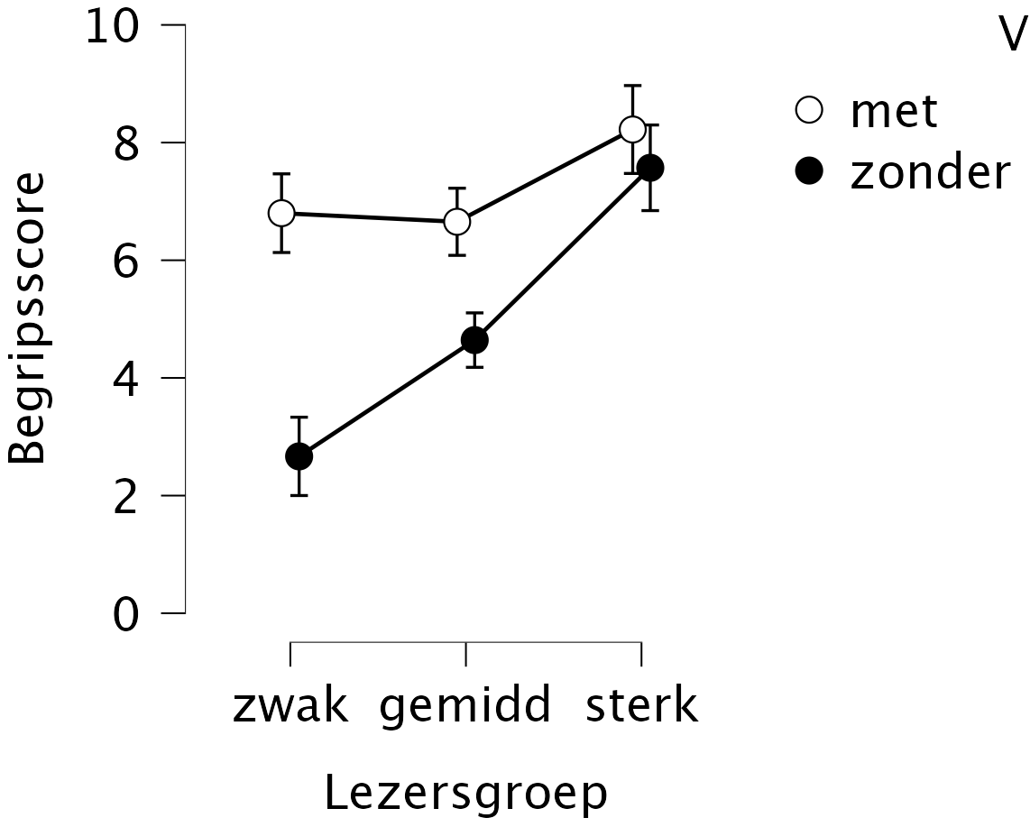
Average comprehension score (along Y axis, with 95% confidence intervals), for text versions with (met) and without (zonder) structure markers, for weak (zwak), average (gemidd) and strong (sterk) readers (after Van Dooren, Van den Bergh and Evers-Vermeul, 2012).

Figure 15.3: Average comprehension score (along Y axis, with 95% confidence intervals), for text versions with (met) and without (zonder) structure markers, for weak (zwak), average (gemidd) and strong (sterk) readers (after Van Dooren, Van den Bergh and Evers-Vermeul, 2012).

If a significant interaction is present, as in the example above, then we can no longer draw conclusions about the main effects involved in that interaction. This is because the effect of a factor now depends on the levels of the other factor, i.e., on the interaction with other factor(s) ³⁷. In the example above: the difference in comprehension scores between the text versions (factor A) is large for weak readers, but absent for strong readers. The difference between reader types (factor B) is larg for a text without markers, but far smaller for a text with structural markers.

We have already seen a different pattern of interaction, in Figure 6.1 (§6.8). There, the scores are on average about the same for the two groups of listeners, and on average the scores are about the same for the two conditions too. Hence the two main effects are not significant, but their interaction is highly significant. In that study, the effect of the one factor is opposite in the two levels of the other factor.

15.4.2 A formal explanation

We again assume that the scores have been built up according to a statistical model, namely as the sum of the population mean \(\mu\), a systematic effect \(\beta_k\) of the \(k\)’the condition of factor B, a systematic effect \((\alpha\beta)_{jk}\) of the combination of conditions \((j,k)\) of factors A and B, and a chance effect \(e_{ijk}\) for the \(i\)’the replication within the \(jk\)’the cell. In formula:

\[x_{ijk} = \mu + \alpha_{j} + \beta_{k} + (\alpha\beta)_{jk} + e_{ijk}\]

In the one-way analysis of variance the total ‘sums of squares’ is split up into two components, namely between and within conditions (see equation (15.4)). With the two-way analysis of variance, there are now however four components, viz. three between conditions and one within conditions (within):

\[\begin{equation} \tag{15.8} { SS_t } = SS_A + SS_B + SS_{AB} + SS_{within} \end{equation}\]

\[\begin{align} \tag{15.9} { \sum (x_{ijk} - \overline{x})^2 } = & { \sum_j n_j (\bar{x}_j - \bar{x})^2 } + \\ & { \sum_k n_k (\bar{x}_k - \bar{x})^2 } + \\ & { \sum_j \sum_k n_{jk} (\bar{x}_{jk} - \bar{x}_j - \bar{x}_k + \bar{x})^2 } + \\ & { \sum_i \sum_j \sum_k (x_{ijk} - \bar{x}_{jk})^2 } \end{align}\]

The degrees of freedom of these sums of squares also add up to each other again: \[\begin{align} \tag{15.10} { (N-1) } &= (A-1) &+ (B-1) &+ (A-1)(B-1) &+ (N-AB) \\ \textrm{df}_t &= \textrm{df}_A &+ \textrm{df}_B &+ \textrm{df}_{AB} &+ \textrm{df}_{within} \end{align}\]

Just as with the one-way analysis of variance, we again calculate the ‘mean squares’ by dividing the sums of squares by their degrees of freedom.

We now test three null hypotheses, namely for the two main effects and their interactions. For each test, we determine the corresponding \(F\)-ratio. The numerator is formed from the observed variance, as formulated above; the denominator is formed from \(s^2_w\), the chance variance between the replications within the cells. All the necessary calculations for analysis of variance, including determining the degrees of freedom and p-values, are carried out by computer nowadays.

The results are summarised again in an ANOVA table, which has now been somewhat extended in Table 15.5. We now test and report three hypotheses.

Table 15.5: Summary of two-way analysis of variance (ANOVA) of the comprehension scores of two text versions and three reader types.
source	df	SS	MS	\(F\)	\(p\)
(A) text version	1	91.2663	91.2663	63.75	<.001
(B) reader type	2	96.0800	48.0400	33.56	<.001
(C) interaction	2	30.7416	15.3708	10.74	<.001
within	88	125.9830	1.4316

It is customary to present the results of the main effects before the interaction effects. For the interpretation, it matters whether or not the interaction is significant. If the interaction is significant, then first we present the main effects without interpreting them, then we present and interpret the interaction, and finally we interpret the main effects that are significant and that are not involved in the interaction. If the interaction is not significant, then it may be easier to first present and interpret the main effects, and then we present the interaction (which is not interpreted).

15.4.3 Post hoc comparisons

In two-way ANOVA too, we can perform post hoc comparisons (cf. §15.3.5) to investigate which cells or conditions differ from each other. Again we use the Tukey HSD test, which provides a 95% confidence interval of the difference between two cells, and/or a \(p\) value of that difference.

The comprehension scores showed a significant main effect of structure markings in the text \([F(1,88)=63.75, p<.001, \omega^2=0.26]\), as well as a significant main effect of the reader type \([F(2,88)=33.56, p<.001, \omega^2=0.27]\). There was also a significant interaction between text version and reader type \([F(2,88)=10.74, p<.001, \omega^2=0.08]\), see Figure 15.3; this interaction was further explored using the Tukey HSD test (among 6 cells). Weak readers perform worse than average readers, in the text version without markers (\(p<.001\)), but not in the version with markers (\(p=.99\)). Strong readers perform better than average readers, in the version without markers (\(p<.001\)) as well as with markers (\(p=.01\)). Text markers have an effect for weak readers (\(p<.001\)) and for average readers (\(p<.001\)) but not for strong readers (\(p=.89\)); hence strong readers do not benefit from structure markers in the text, but weak and average readers do. Also of interest is the finding that weak readers understand a text with markers as well as strong readers do understand the same text without markers (\(p=.72\)).

15.4.4 SPSS

The data for the example above are in data/DBE2012.csv.

15.4.4.1 ANOVA

Analyze > General Linear Model > Univariate...

Drag the dependent variable (MCBiScore) to the panel Dependent variable. Drag the two independent variable (with Dutch variable names, Versie for text version, Groep for group or reader type) to the panel Fixed factor(s).

15.4.5 JASP

15.4.5.1 preparation

The data for the example above are in data/DBE2012.csv.

Examine whether the responses are normally distributed within each group or cell, using the techniques from Part II of this textbook (especially §10.4). Note: In JASP it is possible to examine the distribution at the same time as the analysis of variance itself, see below.

15.4.5.2 ANOVA

In the top menu bar, choose:

ANOVA > Classical: ANOVA

Select the variable MCBiScore and move it to the field “Dependent Variable”, and move the variables Version (text version) and Group (reader type) to the field “Fixed Factors”.
Under the heading “Display” check Estimates of effect size, and select \(\omega^2\) and/or (partial) \(\eta^2\). In this book we prefer \(\omega^2\). You can also check Descriptive statistics to learn more about the scores in each cell.

Open the menu bar named “Model” and for “Sum of squares” choose option Type III.
Open the menu bar named “Assumption Checks” and check Homogeneity tests.
“Homogeneity corrections” may remain at the default value of None. Here you can also examine whether the distribution within each group or cell is normal, as assumed by the analysis of variance. This is equivalent to assuming a normal distribution of the residuals of the analysis of variance. You can inspect the latter by checking Q-Q plot of residuals. If the assumption is met (and if residuals are distributed normally) then the residuals should fall on an approximately straight line in the resulting Q-Q plot (see §10.4).
Open the menu bar named “Descriptive Plots” and select Group for the field “Horizontal Axis” and select Version for the field “Separate Lines”.

The output summarizes the analysis of variance in a table similar to Table 15.5, with the effect size included. The Descriptive plots section provides a visualisation which may be helpful in understanding a possible interaction effect.

The output under Assumption Check also reports Levene’s test for equal variances (homogeneity of variance). This test does not suggest rejection of H0, so we may conclude that the variances are indeed approximately equal, i.e., that that particular assumption of the analysis of variance is warranted.

15.4.5.3 post hoc comparisons

For an analysis of variance with post-hoc comparisons we need to specify the post-hoc comparisons. The procedure is initially the same as above, so repeat the instructions given under ANOVA above.

Next, open the bar named “Post Hoc Tests”, and move the interaction Versie \(\times\) Groep to the righthand field. Check that “Type” is set to Standard and that the option Effect size is also checked. Under “Correction” check the option Tukey, and under “Display” check the option Confidence intervals.

For the version without markers (‘zonder’) we see that the cell zonder:zwak scores lower than the cell zonder:gemiddeld (\(p<.001\)), and that the cell zonder:sterk scores higher than the cell zonder:gemiddeld (\(p<.001\)). For the version with markers (‘met’) we see that the cell met:zwak scores about equally with the cell met:gemiddeld (\(p=.99\)), and that the cell met:sterk scores higher than the cell met:gemiddeld (\(p=.01\)). Hence strong readers perform better than average and/or weak readers, in both text versions. We also see that zonder:zwak scores lower than met:zwak (\(p<.001\)), and that zonder:gemiddeld scores lower than met:gemiddeld (\(p<.001\)), while there is no difference between zonder:sterk and met:sterk (\(p=.89\)). Hence strong readers do not benefit from structure markers in the text. Also of interest is the finding that weak readers understand a text with markers as well as strong readers do understand a text without markers (\(p=.72\)).

15.4.6 R

15.4.6.1 preparation

The data for the example above are in data/DBE2012.csv.

DBE2012 <- read.csv(file="data/DBE2012.csv")
# Versie: 1=with=met, 2=without=zonder structure markers
# Groep: 1=weak=zwak, 2=average=gemiddeld, 3=strong=sterk
# ensure that Versie and Groep are factors, levels are in Dutch here
DBE2012$Versie <- factor(DBE2012$Versie, labels=c("met","zonder") ) 
DBE2012$Groep <- factor(DBE2012$Groep, labels=c("zwak","gemiddeld","sterk") )
# DV: MCBiScore: number of comprehension questions (out of 10) 
#     that were answered correctly, from a biology text
# make table of means, see Figure 15.3
with( DBE2012, tapply( MCBiScore, list(Versie,Groep), mean ))

##            zwak gemiddeld    sterk
## met    6.800000  6.653846 8.222222
## zonder 2.666667  4.642857 7.571429

15.4.6.2 ANOVA

summary( aov(MCBiScore~Versie*Groep, data=DBE2012) -> DBE2012.m1 )

##              Df Sum Sq Mean Sq F value   Pr(>F)    
## Versie        1 121.18  121.18   84.64 1.59e-14 ***
## Groep         2  81.41   40.71   28.43 2.98e-10 ***
## Versie:Groep  2  30.74   15.37   10.74 6.72e-05 ***
## Residuals    88 125.98    1.43                     
## ---
## Signif. codes:  0 '***' 0.001 '**' 0.01 '*' 0.05 '.' 0.1 ' ' 1

The results are slightly different from those reported in Table 15.5 above, because R computes the sums of squares somewhat differently³⁸.

15.4.6.3 Effect size

In order to assess effect size, we will use the previously programmed function omegasq (§15.3.8.3):

omegasq(DBE2012.m1, "Versie")        # [1] 0.33

## [1] 0.3319423

omegasq(DBE2012.m1, "Groep")         # [1] 0.22

## [1] 0.2177437

omegasq(DBE2012.m1, "Versie:Groep")  # [1] 0.08

## [1] 0.07727868

These results too differ slighly from those reported in the main text above, because R computes the sums of squares somewhat differently.

15.4.6.4 post-hoc tests

TukeyHSD(x=DBE2012.m1, which="Versie:Groep")

##   Tukey multiple comparisons of means
##     95% family-wise confidence level
## 
## Fit: aov(formula = MCBiScore ~ Versie * Groep, data = DBE2012)
## 
## $`Versie:Groep`
##                                      diff         lwr        upr     p adj
## zonder:zwak-met:zwak           -4.1333333 -5.60315087 -2.6635158 0.0000000
## met:gemiddeld-met:zwak         -0.1461538 -1.27642935  0.9841217 0.9989799
## zonder:gemiddeld-met:zwak      -2.1571429 -3.27255218 -1.0417335 0.0000031
## met:sterk-met:zwak              1.4222222 -0.04759532  2.8920398 0.0637117
## zonder:sterk-met:zwak           0.7714286 -0.82423518  2.3670923 0.7218038
## met:gemiddeld-zonder:zwak       3.9871795  2.63899048  5.3353685 0.0000000
## zonder:gemiddeld-zonder:zwak    1.9761905  0.64044018  3.3119408 0.0005900
## met:sterk-zonder:zwak           5.5555556  3.91224959  7.1988615 0.0000000
## zonder:sterk-zonder:zwak        4.9047619  3.14799393  6.6615299 0.0000000
## zonder:gemiddeld-met:gemiddeld -2.0109890 -2.96040355 -1.0615745 0.0000003
## met:sterk-met:gemiddeld         1.5683761  0.22018706  2.9165651 0.0130213
## zonder:sterk-met:gemiddeld      0.9175824 -0.56680056  2.4019654 0.4704754
## met:sterk-zonder:gemiddeld      3.5793651  2.24361478  4.9151154 0.0000000
## zonder:sterk-zonder:gemiddeld   2.9285714  1.45547670  4.4016662 0.0000016
## zonder:sterk-met:sterk         -0.6507937 -2.40756162  1.1059743 0.8883523

These results too differ slighly from those reported in the main text above, because R computes the sums of squares somewhat differently.

For each pairwise comparison among the 2x3 cells we see the difference, the lower and upper boundary of the 95% confidence interval of the difference, and the adjusted \(p\) value using Tukey’s HSD correction.

References

Kerlinger, Fred N., and Howard B. Lee. 2000. Foundations of Behavioral Research. 4th ed. Fort Worth: Harcourt College Publishers.

Maxwell, Scott E., and Harold D. Delaney. 2004. Designing Experiments and Analyzing Data: A Model Comparison Perspective. Book. 2nd ed. Mahwah, NJ: Lawrence Erlbaum Associates.

Olejnik, Stephen, and James Algina. 2003. “Generalized Eta and Omega Squared Statistics: Measures of Effect Size for Some Common Research Designs.” Psychological Methods 8 (4): 434–47.

Quené, Hugo. 2008. “Multilevel Modeling of Between-Speaker and Within-Speaker Variation in Spontaneous Speech Tempo.” Journal of the Acoustical Society of America 123 (2): 1104–13.

Van Dooren, Wendy, Huub Van den Bergh, and Jacqueline Evers-Vermeul. 2012. “Leesbare Teksten? Over de Invloed van Structuurmarkeringen Op Het Tekstbegrip En Tekstwaardering van Zwakke En Sterke Lezers.” Levende Talen Tijdschrift 13 (4): 31–38. https://lt-tijdschriften.nl/ojs/index.php/ltt/article/view/152.

If (1) red does differ from grey and blue, and if (2) grey and blue also differ from each other, then this implies that red differs from grey (a new finding) and that red differs from blue (we already knew that).↩︎
If we add more factors then the situation quickly becomes confusing. With three main effects, there are already 3 two-way interactions plus 1 three-way interaction. With four main effects, there are already 6 two-way interactions, plus 4 three-way interactions, plus 1 four-way interaction.↩︎
The default type of computing sums of squares in R (Type I) may be used in JASP by choosing: Model, Sum of squares: Type I. The default type of computing sums of squares in JASP (Type III) may be achieved in R by various workarounds, see e.g. https://www.r-bloggers.com/2011/03/anova-%E2%80%93-type-iiiiii-ss-explained.↩︎