14 Power
14.1 Introduction
With statistical testing of H0, we determine the probability \(P\) of the observed differences or effects (or of even larger differences or effects than observed) if H0 were true, and thus if the observed difference had to be attributed solely to chance (see §2.5 and Chapter 13). If the probability \(P\) is very small, then we have thus found results which are very improbable if H0 were true. We then conclude that H0 is presumably not true and we thus reject H0. We then call the difference or effect found, the “significant” (Latin: ‘meaning making’). However, there is in fact a probability, \(P\), that the difference found is actually a fluke, and that, by rejecting H0, we are making a Type I error (i.e. wrongly rejecting H0, see §13.1). As we use a certain significance level, with which to compare \(P\), this \(\alpha\) is thus also the probability that we are making a Type I error.
At least as important, however, is the opposite error of not wrongly
rejecting H0, a Type II error. Examples of such errors are:
not convicting a suspect even if he is guilty, letting a ‘spam’
email message through into my mailbox, examining a patient and nevertheless
not noticing their illness, concluding that birds are silent when
they are in fact singing
(Example 13.1), or wrongly concluding that two
groups do not differ when an important difference does in fact exist
between the two groups. The probability of a Type II error is referred to
with the symbol \(\beta\).
If H0 is in fact not true (there is a difference, the message is ‘spam’, birds are singing, etc.), then H0 should be rejected, and \(\beta\) should thus be as small as possible. The probability of rightly rejecting H0 is then \((1-\beta)\) (see complement rule (10.3)); this probability \((1-\beta)\) is called the power. Power can be interpreted as the probability of the researcher being right (H0 is rejected) when she is indeed right (H0 is untrue).
The probabilities of Type I and Type II errors have to be weighed up carefully against each other. In many studies, the p-values \(\alpha=.05\) (significance level) and \(\beta=.20\) (power=\(.80\)) are used. With these, an implicit weighting is made that a Type I error is 4× more grave than a Type II error. For some studies that might be justified but it is also easily conceivable that, under certain circumstances, a Type II error is actually more grave or serious than a Type I error. If we find both types of error more or less equally grave, then we should strive for a smaller \(\beta\) and larger power (Rosenthal and Rosnow 2008).
The power of a study depends on three factors: (i) the effect size \(d\), which itself is in turn dependent on the measured difference \(D\) and the variation \(s\) in the observations (formula (13.9)), (ii) the sample size \(N\), and (iii) the significance level \(\alpha\). In the following sections, we will discuss each of these factors separately, and, when doing so, keep the other two factors as constant as possible. For this discussion, we will use the depictions of calculated power (Figures 14.1 and 14.2). The depicted power contours are specifically for a t-test for independent samples (§13.6) with two-sided testing. The relations discussed below also apply to other statistical tests.
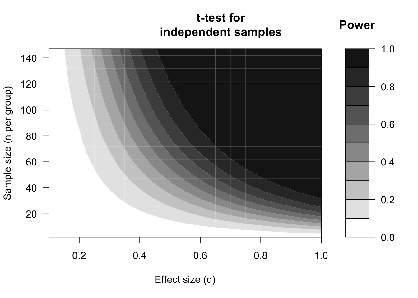
Figure 14.1: Power expressed in contours (see shading), dependent on the standardised effect size (d) and sample size according to a two-sided t-test for unpaired, independent observations, with two-sided significance level alpha=.01.
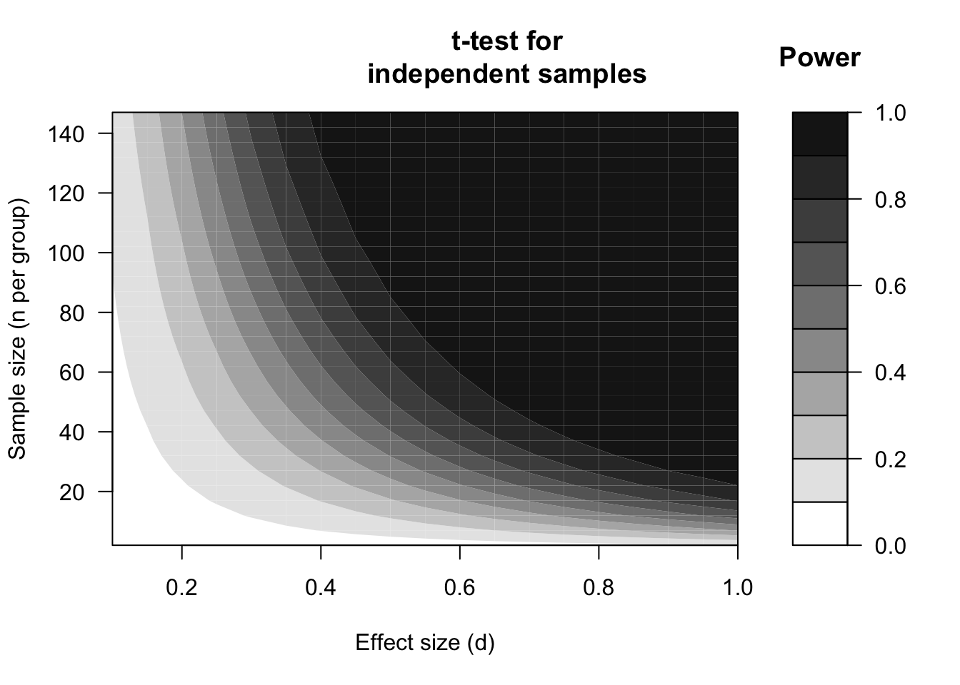
Figure 14.2: Power expressed in contours (see graduation), dependent on the standardised effect size (d) and the sample size (n), according to a two-sided t-test for unpaired, independent observations with significance level alpha=.05.
14.2 Relation between effect size and power
The two figures 14.1 and 14.2 show that, in general, the larger the effect to be tested is (more to the right in each figure), the larger the power. This is also not surprising: a larger effect has a higher probability of being detected in a statistical test, under the same circumstances. A moderately large effect of \(d=.5\), with \(n=30\) observations in each group, only has a probability of \(.48\) of being detected (if \(\alpha=.05\), Figure 14.2). On the basis of a study with \(n=30\) observations per group is thus actually a gamble whether a researcher will actually detect such an effect, and will reject H0. Put otherwise, the probability of a Type I error is admittedly safely low (\(\alpha=.05\)) but the probability of a Type II error is more than \(10\times\) as large, and thus dangerously high (\(\beta=.52\)) (Rosenthal and Rosnow 2008, Ch.12).
A larger effect has a higher probability of being detected. A larger effect of \(d=.8\), for example, results in a power of \(.86\) with this testing. The probability of a Type II error \(\beta=.14\) here is admittedly also larger than the probability of a Type I error, but the proportion \(\beta/\alpha\) is considerably less skewed.
As researchers, we only have an indirect influence on effect size. We of course have no influence on the true raw difference \(D\) in the population. For the power, however, the raw difference \(D\) is not important, but rather the standardised difference \(d=D/s\) (§13.8). Thus, if we ensure that the standard deviation \(s\) decreases, then \(d\) will increase, and then the power will also increase (figures 14.1 and 14.2), and we thus have a higher probability of actually detecting an effect! With this goal in mind, researchers always strive to neutralise disrupting influences from all kinds of other factors as much as possible. After all, the disrupting influences produce extra variability in the observations, and, with this, a lower power with the statistical testing.
In a well-designed study, we want to determine in advance what the power will be, and how large the sample should be (see below). For this we need an estimation of the smallest effect size \(d\) which we still want to detect (§13.8) (Quené 2010). To estimate the effect size, firstly, an estimate of the raw difference \(D\) between the groups or conditions is needed. Secondly, an estimation is needed of the variability \(s\) in the observations. These estimations can be largely deduced from earlier publications, in which the standard deviation \(s\) is usually reported. If no earlier research reports are available, then \(s\) can be roughly estimated from some informal ‘pilot’ observations. Take the difference between the highest and the lowest (range) of these, divide this range by 4, and use the outcome of this as a rough estimation for \(s\) (Peck and Devore 2008).
14.3 Relation between sample size and power
The relation between the sample size \(N\) and the power of a study is illustrated in Figure 14.1 for a strict significance level \(\alpha=.01\), and in Figure 14.2 for the most used significance level \(\alpha=.05\). The figures show that, in general, the larger the sample gets (further upwards), the larger the power is. The increase is steeper (power increases more quickly) with larger effects (right-hand side) than with smaller effects (left-hand side). Put differently: with small effects, the sample is actually always too small to detect these small effects with sufficient power. We already saw that in Example 13.3 (Chapter 13).
The two figures 14.1 and 14.2 are based on the comparison between two groups which are equally large, each with precisely half of the observations (\(n_1=n_2=N/2\)). That is also most efficient. The power is based on the harmonic mean of \(n_1\) and \(n_2\) (see §9.3.4), and that harmonic mean is always smaller than the arithmetic mean of those two numbers. It is thus advisable to ensure that the groups or samples which you compare are approximately equally large.
Example 14.1: In a study, two groups of participants are compared, with \(n_1=10\) and \(n_2=50\)
(\(N=n_1+n_2=10+50=60\)). The harmonic mean of \(n_1=10\) and \(n_2=50\) is \(H=17\). This study thus has the same power as a smaller study with two groups, each of 17 participants, thus 34 participants in total. For this study, thus, 26 participants more have been investigated (and bothered) than necessary (see also §3.2) (Aron, Coups, and Aron 2011, 295).
14.4 Relation between significance level and power
The relation between the significance level \(\alpha\) and the power is illustrated by the difference between the two figures 14.1 and 14.2. For each combination of effect size and sample size, the power is lower in Figure 14.1 for \(\alpha=.01\) than in Figure 14.2 for \(\alpha=.05\). If we choose a higher significance level \(\alpha\), then the probability of rejecting H0 increases, and thus also the power of correctly rejecting H0 when H0 is untrue (see Table 2.2). However, unfortunately, with a high significance level \(\alpha\), the probability of wrongly rejecting H0 (i.e. of making a Type I error) also increases. The investigator must make a well-considered decision between Type I errors (with probability \(\alpha\)) and Type II errors (with probability \(\beta\)); as said earlier, this decision has to depend on the seriousness of (the consequences of) these two types of errors.
14.5 Disadvantages of insufficient power
Unfortunately, many examples can be found of ‘underpowered’ research in the domain of language and communication. This research has a too small probability of rejecting H0 when the investigated effect indeed exists (H0 is not true). Why is that bad (Quené 2010)?
Firstly, the Type II error which occurs here can have serious consequences: a treatment method which is actually better is not recognised as such, a patient is not or wrongly diagnosed, a useful innovation is wrongly pushed aside. This error hinders the growth of our knowledge and our insight, and hinders scientific progress (see also Example 3.2 in Chapter 3).

Figure 14.3: Effect sizes (along the horizontal axis) found in simulated experiments (two-sided t-test for independent observations, alpha=.05), broken down according to sample size (left \(n=20\), right \(n=80\)) and according to testing result (dark symbols: significant; light symbols: not significant). The true effect size between groups is always \(d=0.5\), indicated by the grey dashed line. The mean effect size found from the significant outcomes is referred to with the black dashed line. For each sample size, 100 simulations have been carried out (long vertical axis).
The outcomes of simulated experiments with different sample size, and thus with different power, are summarised in Figure 14.3. We explain the second disadvantage on the basis of the somewhat complex figure. In the left panel of Figure 14.3, we can see that the different (simulations of) ‘underpowered’ studies show a mixed picture. Some of these studies do show a significant effect (dark symbols), and many other studies do not (light symbols). The mixed picture then usually leads to follow up research, in which people try to find out why the effect does occur in some studies, and not in others. Might the difference in results be attributable to differences in stimuli? participants? tasks? instruments? All that follow up research is superfluous though: the mixed picture from these studies can be explained by the small power of each study. The needless and superfluous follow up research costs much time and money (and indirect costs, see Chapter 3), and comes at the cost of other, more useful research (Schmidt 1996, 118). Put otherwise: one well designed study with power which is more than sufficient can avoid many needless follow up studies.
The third disadvantage is based on the experience that studies in which a significant effect is found (dark symbols) have a higher probability of being reported; this phenomenon is called ‘publication bias’ or the ‘file drawer problem’. After all, a positive result often does get published, whilst a negative result often disappears into a file drawer. With small power, that leads to the third disadvantage, namely an overestimation or ‘bias’ of the reported effect size. In an underpowered study, after all, an effect must be quite large to be found. In the leftmost panel, we can see that a significant effect has only been found \(31\times\). The average effect size of these 31 significant outcomes is \(\overline{d_{\textrm{signif}}}=0.90\) (black dashed line), i.e. a distortion or ‘bias’ of \(0.40\) relative to the actual \(d=0.50\) (grey dashed line)35. In the rightmost panel, we can see that a significant effect has been found \(91\times\) (thus the power here is sufficient). The mean effect size of these 91 significant outcomes hardly deviates from the actual \(d\). Moreover, the standard deviation of the reported effect size is smaller, and that is again important for later research, meta-studies, and systematic reviews.
Fourthly, the mixed picture from the different studies, sometimes with significant outcomes and sometimes without, and with great variation in the reported effect size, carries the danger that these outcomes are taken less seriously than ‘consumers’ of scientific knowledge (practitioners, health insurers, developers, policy makers, etc.). In this way, these consumers get the impression that the scientific evidence for this investigated effect is not strong, and/or that the researchers are in disagreement about whether the effect exists and if it does, how large it then is (Van Kolfschooten 1993) (Figure 14.3). This, also hinders scientific progress, and it hinders the use of scientific insights in societal applications.
To avoid all these objections, researchers have to take into account the desired power of a study in an early stage. Designing and conducting a study with insufficient power is after all in opposition with the earlier discussed ethical and moral principles of diligence and responsibility (§3.1).
References
A replication study which does have sufficient power, thus typically finds a smaller effect than the original ‘underpowered’ study. The smaller effect found in the replication study is then typically also not significant. We then say that the replication study “fails to replicate” the effect that was significant in the original study - but that was actually a spurious finding.↩︎