13 Testing hypotheses
13.1 Introduction
From this chapter onwards, we will be concerned with the testing of research hypotheses and, in particular, with null hypothesis significance testing (NHST), as explained in Chapter 2.
Over the course of the years, a large number of techniques have been developed for tests like this. The tests with which we will concern ourselves are the most used and can be divided into parametric and non-parametric tests. Parametric tests assume that the dependent variable is (at least) measured on an interval level of measurement (see Chapter 4), and that the measured outcomes or scores are normally distributed (see §10.3 and §10.5). For non-parametric tests, dependent on the technique, fewer assumptions are made over the level of measurement or over the distribution of the observed scores; these are so-called distribution free tests. The consequence is that the testing is a little less ‘sensitive’ under otherwise equal circumstances, i.e. that the null hypothesis can be rejected less often in otherwise equal circumstances. These tests therefore have less power (see Chapter 14). Researchers thus usually prefer parametric tests.
We already discussed the general principle of testing briefly in
§2.4 and §2.5.
We will illustrate this once more here
with an example. We investigate the statement H1:
‘Linguistics students master traditional grammar better than the average language student’.
As a measurement instrument, we use the so-called “grammar test”33 which is compulsory
for most students
in language programs at Utrecht University. On the basis of previous cohorts (year groups),
we expect a mean score of 73 on this test;
this is the mean number of correct answers to 100 questions.
We thus operationalise H1 as \(\mu > 73\), and from this deduce
the accompanying null hypothesis which is actually tested:
\(\mu = 73\).
(In §13.4 below, we will go into more detail
about whether or not to specify the direction of the difference in H1).
For a sample consisting of the first year Linguistics students (\(n=34\)) from a certain cohort, we find an average score of 84.4. That is indeed far above the reference value of 73 — but that might also be a coincidence. Perhaps, H0 is true, and, by chance, there happen to be many grammar experts in our sample (from the population of possible first year students in Linguistics). We can calculate the probability \(P\) of this situation, i.e. the probability \(P\) of finding a mean score of \(\overline{x}=84.4\), given a random sample of \(n=34\) participants and given that H0 is in fact true (i.e. \(\mu=73\)): this probability \(P=.000000001913\). This probability \(P\) represents the probability of finding this data, whilst H0 is true: \(P(\overline{x}=84.4|\textrm{H0}, n=34)\). In this example, the probability \(P\) is very small.
For the argumentation, it is essential that the data are valid and reliable — this is precisely the reason why we discussed validity (Chapter 5) and reliability (Chapter 12). If we have done everything properly, we may, after all, trust the data obtained. We are then not able to attribute the low \(P\) (probability of the data according to H0) to errors in operationalisation, or to measurement errors, or to other deviations or artefacts in the data. The logical conclusion then must be that the improbable outcome shows that the premise (H0) is probably not true: we reject H0; H0 has thus been falsified. Thereby, our knowledge has increased because we can now assume on legitimate grounds that H0 is untrue (and thus that H1 must be true).
If we reject H0 on the basis of the reasoning above which in turn is based on probability, then we do have to take into account the small probability \(P\) that rejecting H0 is an incorrect decision (Type I error; see §2.5). After all, there is the probability \(P\) that we find these data when H0 is in fact true (in this example: when the linguists on average do not score better than \(\mu=73\)).
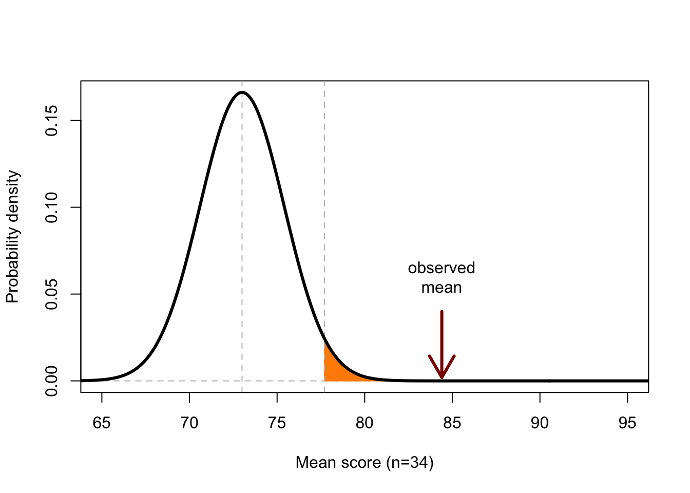
Figure 13.1: Probability distribution of the mean score from a sample (n=34) with a population mean 73 and population s.d. 14. The coloured area covers 5% of the total area under the curve; outcomes along the X-axis of this area thus have a probability of at most 5% of occurring if H0 is true.
Figure 13.1 shows the probability of the sample mean (\(n=34\)) if H0 is true. We see that the value 73 has the highest probability, but also 72 or 74 are probable mean scores according to H0. However, a mean of 84.4 is very improbable: the probability \(P\) of observing this mean score, or a higher score (area under the curve, to the right of the observed mean) is almost null according to H0.
The boundary value for \(P\), at which we reject H0 is called the significance level, often referred to with the symbol \(\alpha\) (see §2.5). Researchers often use \(\alpha=.05\), but sometimes other boundary values are also used. In Figure 13.1, you see that the probability of a mean score of 77.7 or more has a probability of \(P=.05\) or smaller, according to H0. This can be seen from the area under the curve. The coloured part has precisely an area of 0.05 or 5% of the total area under the curve.
The decision about whether or not to reject H0 is based on the probability \(P\) of the outcomes, given H0. The decision might also be incorrect. The finding that \(P < \alpha\) is thus not an irrefutable proof that H0 is untrue (and has to be rejected); it could also be that H0 is in fact true but that the effect found was a fluke (Type I error). Conversely, the finding that \(P > \alpha\) is not conclusive evidence that H0 is true. There can be all kinds of other, plausible reasons why an effect which exists (H0 is untrue) can still not be observed. If I do not hear any birds singing, that does not necessarily mean that there are genuinely no birds singing. More generally: “absence of evidence is not evidence of absence” (Sagan 1996, 121; Alderson 2004). It is therefore recommended to always report the size of the effect found; this is explained in more detail in §13.8 below.
Example 13.1: Assume H0: ‘birds do not sing’. Write down at least 4 reasons why I do not hear birds singing, even if there are in fact birds singing (H0 is untrue). If I do not reject H0, what type of error will I be making?
13.2 One-sample \(t\)-test
The Student’s \(t\)-test is used to investigate a difference between the mean score of a sample, and an a priori assumed value of the mean. We use this test when the standard deviation \(\sigma\) in the population is unknown, and thus has to be estimated from the sample. The line of thought is as follows.
We determine the test statistic \(t\) on the basis of the mean and the
standard deviation in the sample, and of the assumed mean (according to H0).
If H0 is true, then the value \(t=0\) is the most
probable. The larger the difference between the observed sample mean and the
assumed sample mean, the more \(t\) increases. If the test statistic \(t\) is larger than
a certain boundary value \(t*\), and thus \(t>t*\), then the probability of this test statistic,
if H0 is true, is very small: \(P(t|\textrm{H0}) < \alpha\). The probability of finding this result
if H0 is true is then so small that we decide to reject H0
(see §2.5). We speak then of a significant difference:
the deviation between the observed and the expected mean is probably not a
coincidence.
In the earlier example of the grammar test with Linguistics students (§13.1), we already became acquainted with this form of \(t\)-test. If \(\overline{x}=84.4, s=8.4, n=34\), then the test statistic is \(t=7.9\) according to formula (13.1) below.
The probability distribution of test statistic \(t\) under H0 is known; you can find the boundary value \(t^*\) in Appendix C. Put otherwise, if the test statistic \(t\) is larger than the boundary value \(t^*\) which is stated in the table then \(P(t|\textrm{H0})<\alpha\). To be able to use the table in Appendix C, we still have to introduce a new term, namely the number of degrees of freedom. That term is explained in §13.2.1 below.
With the number of degrees of freedom, you can look in Appendix
C to see which boundary value \(t^*\) is needed
to achieve a certain p-value for the established test statistic
\(t=7.9\). Let us see what the p-value is for the established
test statistic \(t=7.9\). We firstly look for the degrees of freedom (‘d.f.’) in the left column.
If the number of degrees of freedom does not occur in the table, then, to err
on the side of caution, we should round down, here to 30 d.f. This determines the row
which is applicable for us. In the third column, we find \(t^*=1.697\). Our
established test statistic \(t=7.9\) is larger than this \(t^*=1.697\), thus the p-value
is smaller than the \(p=.05\) from the third column. If we go further right on
the same line, we see that the stated \(t^*\) increases further.
Our established test statistic \(t\) is even larger than \(t^*=3.385\) in the last column.
The p-value is thus even smaller than \(p=.001\) from the title of that last
column. (The statistical analysis program usually also calculates the p-value.)
We report the result as follows:
The mean score of Linguistics students (cohort 2013) is 84.4 (\(s=8.4\)); this is significantly better than the assumed population mean of 73 \([t(33)=7.9, p<.001]\).
13.2.1 Degrees of freedom
To explain the concept of degrees of freedom, we begin with an analogy. Imagine that there are three possible routes for getting from A to B: a coast path, a mountain path, and a motorway. A walker who wants to travel from A to B has three options, but there are only two degrees of freedom for the walker: he or she only has to make two choices to choose from the three options. Firstly, the motorway option is discarded (first choice), and then the mountain path is discarded (second choice), after which the coast path is the only option remaining. Thus there are two ‘free’ choices, in order to choose one of the three possible routes. If we know the two choices, then we can deduce which route must have been chosen.
Now, we will look at a student who on average has achieved a \(\overline{x}=7.0\) over the \(N=4\) courses from the first introductory track of his or her degree programme. The mean of \(7.0\) can be arrived at in many ways, e.g. \((8,7,7,6)\) or \((5,6,8,9)\). But if we know the result of three of the courses, and we also know that the mean is a 7.0, then we also know what the value of the fourth observation must be. This last observation is thus no longer ‘free’ but is now fixed by the first three observations, in combination with the mean over \(N=4\) observations. We then say that you have \(N-1\) degrees of freedom to determine this characteristic of the sample, such as the sample mean here, or such as the test statistic \(t\). The degrees of freedom is often abbreviated to ‘d.f.’ (symbol \(\nu\), Greek letter “nu”).
In practice, the number of degrees of freedom is not difficult to determine. We indicate for every test how the degrees of freedom are established — and the number of d.f. is usually also calculated and reported by the statistical analysis program that we use.
For the \(t\)-test of a single sample, the number of degrees of freedom is the number of observations \(N-1\). In the above discussed example, we thus have \(N-1 = 34-1 = 33\) degrees of freedom.
13.2.2 formulas
\[\begin{equation} t = \frac{ \overline{y}-\mu} { s } \times \sqrt{N} \tag{13.1} \end{equation}\]
13.2.3 assumptions
The \(t\)-test for a single sample requires three assumptions which must be satisfied in order to be able to use the test.
13.2.4 SPSS
The above discussed data can be found in the file data/grammaticatoets2013.csv.
To test our earlier hypothesis, in SPSS, we firstly have to select the observations of the Linguistics students.
Data > Select cases...Choose If condition is satisfied and click on the button If... to indicate
the conditions for selection (inclusion).
Select the variable progr (drag to the panel on the right-hand side), pick
button =, and then type TW (the Dutch label for “Linguistics”), so that the whole condition is
progr = TW.
Afterwards, we can test our earlier hypothesis as follows:
Analyze > Compare Means > One-Sample T Test...Select variable (drag to the Test variable(s) panel).
Indicate which value of \(\mu\) has to be tested: set it as
Test Value 73. Confirm OK.
The output contains both descriptive statistics and the results of a two-sample \(t\)-test.
When transferring this output, take good note of the warning in
§13.3 below: SPSS reports as if p=.000 but that is untrue.
13.2.5 JASP
The above discussed data can be found in the file data/grammaticatoets2013.csv.
To test our earlier hypothesis, in JASP, we firstly have
to select or filter the observations of the Linguistics students. To do so, go to the data sheet, and click on the funnel or filter symbol in the top left cell. A working panel will appear in which you can specify the selection.
Select the variable progr from the lefthand menu, so that it moves to the working panel. Then click on the symbol = from the top menu of operators, and type TW (the Dutch abbreviation for the Linguistics program, use capitals, no quotes). The complete condition on the working panel should now be progr = TW.
Next click on the button Apply pass-through filter below the working panel in order to apply this filter. In the data sheet, you should see immediately that the rows of excluded data (students of other programs than Linguistics) are greyed out. Those rows (observations) will no longer be used, until you cancel the selection (which is explained below).
To conduct the one sample \(t\) test, choose from the top menu bar:
T-Tests > Classical: One Sample T-TestIn the field “Variables”, select the variable score to be tested.
Under “Tests”, check Student (for Student’s \(t\) test statistic), and as the Test value enter the value of \(\mu\) to use in the test; for this example, enter 73. Under “Alt. Hypothesis”, select > Test value for a one-sided \(t\) test; here we test H1: \(\mu>73\) (see §13.4).
Under “Additional Statistics”, you may check Descriptives and Descriptive Plots to learn more about the dependent variable. Also check the option Effect size (see §13.8 below).
Under the heading “Assumption checks”, finally, check the option Normality (see §10.4).
The output reports the one-sided \(t\) test, including its effect size. The table titled Assumption Checks reports the Shapiro-Wilk test of normality. If checked in the input, descriptive statistics and summary plots are also reported. This visualises the test value (here: 73) relative to the scores of the students of Linguistics.
Note that we have activated a filter to select only the students of Linguistics, and this filter remains in effect until it is deactivated. You can de-activate the filter by navigating to the data sheet, go to the top left corner, go to the filter working panel, and double-click on the trash can or waste bin symbol in the lower right corner. A confirmation text “Filter cleared” should appear, and all observations (rows) in the data sheet should be un-greyed and active.
13.2.6 R
Our hypothesis discussed above can be tested with the following commands:
gramm2013 <- read.csv( file="data/grammaticatoets2013.csv",header=F)
dimnames(gramm2013)[[2]] <- c("score","progr")
# program levels have Dutch labels: TW=Linguistics
with( gramm2013,
      t.test( score[progr=="TW"], mu=73, alt="greater" ) )
##
## One Sample t-test
##
## data: score[progr == "TW"]
## t = 7.9288, df = 33, p-value = 1.913e-09
## alternative hypothesis: true mean is greater than 73
## 95 percent confidence interval:
## 81.97599 Inf
## sample estimates:
## mean of x
## 84.41176The notation 1.913e-09 must be read as the number
\((1.913 \times 10^{-9})\).
13.3 \(p\)-value is always larger than zero
The p-value \(p\) can be very small but it is always larger than zero! In the grammar test example above, we found \(P=.000000001913\), a very small probability but one that is larger than zero. This can also be seen from the tails of the corresponding probability distribution which approach zero asymptotically (see Fig.13.1) but never become completely equal to zero. There is always a minimally small probability of finding an extreme value (or an even more extreme value) from you test statistic in a sample — after all, we are investigating the sample precisely because the outcome of the test statistic cannot be established a priori.
In SPSS, however, the p-value is rounded off, and can then appear as
‘Sig. .000’ or \(p=.000\). This is incorrect.
The p-value or significance is not equal to zero, but has
been rounded down to zero, and that is not the same.
Always report the p-value or significance with the correct
accuracy, in this example as \(p<.001\) (Wright 2003, 125).
13.4 One-sided and two-sided tests
The procedure which we discussed above is valid for one-sided tests. This is to say that the alternative hypothesis does not only put forward that the means will differ but also in which direction that will be: H1: \(\mu >73\), the Linguistics students score better than the population mean. If we were to find a difference in the opposite direction, say \(\overline{x}=68\), then we would not even conceive of statistical testing: the H0 simply still stands. It is only when we find a difference in the hypothesised direction that it is meaningful to inspect whether this difference is significant. When you look now at the figure in Appendix C, then this is also the case. The \(p\)-value corresponds with the area of the coloured region.
If the alternative hypothesis H1 does not specify the direction of the
difference, then a complication arises. Differences in any of the two possible directions
are relevant. We speak then of two-sided tests or two-tailed tests.
To calculate the two-sided p-value, we multiply the \(p\)-value from
Appendix C by \(2\) (because we are now looking at two
coloured regions, on the lower and upper sides of the probability distribution).
In the grammar test example, let us now use a two-sided test. We
then operationalise the alternative hypothesis as H1: \(\mu \ne 73\).
Again, there is \(\overline{x}=73, t=7.9\) with 33 d.f. (rounded off to 30 d.f.).
With the one-sample p-value \(p=.025\) (fourth column), we find
the critical value \(t^*=2.042\). The two-sided p-value
for this critical value is \(2 \times .025 = .05\). The test statistic we found
\(t=7.9\) is larger than this \(t^*=2.042\), thus the two-sided
p-value is smaller than \(p=2\times.025=.05\). The test statistic we found
is larger even than \(t^*=3.385\) in the last column,
thus the two-sided p-value is even smaller than
\(2\times.001\). We can report our two-sided testing as
follows:
The mean score of Linguistics students (class of 2013) is 84.4 (\(s=8.4\)); this observed sample mean differs significantly from the hypothesised population mean of 73 (\(t(33)=7.9, p<.002\)).
In the majority of studies two-sided tests are used; if the direction of the test is not stated then you may assume that two-sided or two-tailed tests have been used.
13.5 Confidence interval of the mean
This section looks more deeply into a subject that was already discussed in §10.7, and illustrates the confidence interval of the mean with the grammar test scores.
We can consider the sample’s mean, \(\overline{x}\), as a good estimation of an unknown mean in the population, \(\mu\). The confidence interval (CI) expresses how (un)trustworthy the estimate is, that is, with what (un)certainty the sample mean, \(\overline{x}\) is related to the population mean \(\mu\) (Cumming 2012). We are familiar with such error margins from election results, where they indicate with what certainty the result of the polling sample (of respondents) matches the actual election result for the entire population (of voters). An error margin of 2% typically means that it is 95% certain that \(x\), the percentage voting for a certain party, will lie between \((x-2)\)% and \((x+2)\)%.
In our example with 30 d.f., we find \(t^*=2.042\) for 95% reliability. Via formula (10.12), we arrive at the 95% confidence interval \((81.5, 87.3)\). What does this confidence interval mean? If we would (and could) draw repeated samples from the same population of Linguistics students, then the reported confidence interval will contain the true population mean for 95% of the repeated samples, and in 5% of the samples the true population mean will be outside the 95% CI. Thus the CI expresses the “confidence in the algorithm and [it is] not a statement about a single CI” (https://rpsychologist.com/d3/ci/).
We report the CI as follows:
The average score of Linguistics students (class of 2013) is 84.4, with 95% confidence interval (81.5, 87.3), 33 d.f.
In Figure 13.2, you can see the results of a computer simulation to illustrate this. This figure is made in the same way as Figure 10.8 in Chapter 10 and illustrates the same point. We have drawn \(100\times\) samples from Linguistics students, with \(\mu=84.4\) and \(\sigma=8.4\) (see §9.5.2) and \(N=34\). For each sample, we have drawn the 95% confidence interval. For 95 of the 100 samples, the population mean \(\mu=84.4\) is indeed within the interval, but for 5 of the 100 samples the confidence interval does not contain the population mean (these are marked along the right hand side). The website https://rpsychologist.com/d3/ci/ shows more of such visual explanations of the concept of confidence intervals.
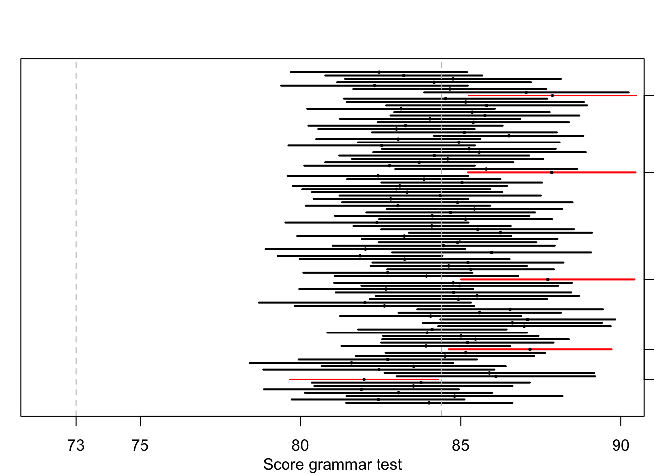
Figure 13.2: 95% confidence interval and sample means, over 100 simulated samples (n=34) from a population with population mean 84.4, population-s.d. 8.4.
From formula (10.12) below, it follows sensibly that if the sample standard deviation \(s\) decreases, and/or if the sample size \(N\) increases, then the confidence interval becomes smaller, i.e., we can be more confident that the observed sample mean is close to the unknown population mean.
13.5.1 formulas
The two-sided confidence interval for \(B\)% reliability for a population mean \(\mu\) is
\[\begin{equation} \overline{y} \pm t^*_{1-B,N-1} \times \frac{s}{\sqrt{N}} \tag{10.12} \end{equation}\]
13.5.2 SPSS
Analyze > Descriptive Statistics > Explore...Select dependent variables (drag to Dependent List panel).
Click on button Statistics and tick Descriptives with Confidence Interval
95%.
Confirm with Continue and with OK.
The output contains several descriptive statistic measures, now also
including the 95% confidence interval of the mean.
13.5.3 JASP
In JASP you can request the confidence interval of the mean by using a one sample \(t\) test. So we conduct this test again and find the confidence interval of the mean in the output.
For the example discussed above, make sure that the proper selection is used so that only observations about students of Linguistics will be included in the analysis (see §13.2.5 for how to filter observations).
Next, from the top menu bar, choose:
T-Tests > Classical: One Sample T-TestIn the field “Variables”, select the variable score to be tested.
Under “Tests”, check Student (for Student’s \(t\) test statistic), and as the Test value now enter \(0\) (zero).
Under “Additional Statistics”, check Location parameter and Confidence interval too. Here you can specify the confidence limits; the default value of 95% is usually OK.
The output reports the mean of score, because observed scores are now compared to the test value which is set to \(0\), so that the Mean Difference of score-0 is now equal to the mean value of score. The same table also reports the 95% CI for Mean Difference, which is equivalent here with the confidence interval of the mean of score.
13.5.4 R
R states the confidence interval of the mean (with self-specifiable confidence level) for a \(t\)-test. We thus again conduct a \(t\)-test and find the confidence interval of the mean in the output.
##
##  One Sample t-test
##
## data:  score[progr == "TW"]
## t = 58.649, df = 33, p-value < 2.2e-16
## alternative hypothesis: true mean is not equal to 0
## 95 percent confidence interval:
##  81.48354 87.33999
## sample estimates:
## mean of x
##  84.41176
13.6 Independent samples \(t\)-tests
The Student’s \(t\)-test is used to allow the investigation of a difference between the mean scores of two independent samples, e.g of comparable boys and girls. On the basis of the mean and the standard deviations of the two samples, we determine the test statistic \(t\). If H0 is true, then the value \(t=0\) is the most probable. The larger the difference between the two means, the larger \(t\) is too. We again reject H0 if \(t>t^*\) for the chosen significance level \(\alpha\).
As a first example, we will take a study of the productive vocabulary size of 18-month old Swedish girls and boys (Andersson et al. 2011). We investigate the hypothesis that the vocabulary of girls differs from that of boys, i.e. H1: \(\mu_{girls} \ne \mu_{boys}\). We cannot a priori assume that a potential difference can only go in one direction; we thus use a two-sided test, as is already evident from H1. The corresponding null hypothesis which we test is H0: \(\mu_{girls} = \mu_{boys}\). In this study, the vocabulary is estimated on the basis of questionnaires from the parents of the children in the sample. Participants were (parents of) \(n_1=123\) girls and \(n_2=129\) boys, who were all 18 months old. Based on the results, it seems that the girls have a mean vocabulary of \(\overline{x_1}=95\) words (\(s_1=82\)), and for the boys it is \(\overline{x_2}=85\) words (\(s_2=98\)). With these data, we determine the test statistic \(t\) according to the formula (13.3), resulting in \(t=0.88\) with 122 d.f. We look for the accompanying critical value \(t^*\) again in Appendix C. In the row for 100 d.f. (after rounding down), we find \(t^*=1.984\) in the fourth column. For two-sample testing we have to double the p-value which belongs to this column (see §13.4), resulting in \(p=.05\). The test statistic \(t < t^*\), thus \(p>.05\). We decide not to reject H0, and report that as follows:
The mean productive vocabulary of Swedish 18-month old Swedish children barely differs between girls and boys (\(t(122)=0.88, p>.4\)). Girls produce on average 95 different words (\(s=82\)), and boys on average 85 different words (\(s=98\)).
As a second example, we take a study of the speech tempo of two groups of speakers, namely originating from the West (first group) and from the North (second group) of the Netherlands. The speech tempo is expressed here as the mean duration of a spoken syllable, in seconds, over an interview of ca. 15 minutes (see Example 15.1). We investigate H0: \(\mu_W = \mu_N\) with two-sample testing. From the results, it appears that those from the West (\(n=20\)) have a mean syllable duration of \(\overline{x_W}=0.235\) s (\(s=0.028\)), and that for those from the North (also \(n=20\)) that is \(\overline{x_N}=0.269\) s (\(s=0.029\)). With these data, we again determine the test statistic \(t\) according to the formula (13.3), resulting in \(t=-3.76\) with 38 d.f. We look for the accompanying critical value again in Appendix C. The correct d.f. are not stated in the table so we round them down (i.e. in the conservative direction) to 30 d.f. In the row, we find \(t^*=2.042\) in the fourth column. For two-sample testing, we have to double the p-value corresponding to these columns (see §13.4), resulting in \(p=.05\). The test statistic is \(t < t^*\), thus \(p<.05\). We thus decide to indeed reject H0, and report that as follows:
The mean duration of a syllable spoken by a speaker from the West of the Netherlands is \(0.235\) seconds (\(s=0.03\)). This is significantly shorter than from speakers from the North of the Netherlands (\(\overline{x}=0.269\) s, \(s=0.03\)) (\(t(38)=-3.76, p<.05\)). In the investigated recordings from 1999, the speakers from the West thus speak more quickly than those from the North of the Netherlands.
13.6.1 assumptions
The Student’s \(t\)-test for two independent samples requires four assumptions which must be satisfied in order to use the test.
The data have to be measured on an interval level of measurement (see §4.4).
All the observations must be independent of each other.
The scores must be normally distributed within each group (see §10.4).
The scores must have approximately equal variances in both groups. The more the two samples differ in size, the more serious the violation of this latter assumption is. It is thus prudent to work with samples that are of (approximately) the same size, and preferably not too small! If the samples are equally large, then the violation of this assumption of equal variances is not so serious (see §13.6.2 directly below).
13.6.2 formulas
13.6.2.1 test statistic
To calculate the test statistic \(t\), various formulas are used.
If the samples have approximately equal variances, then we firstly compute the “pooled standard deviation” \(s_p\) as an intermediate step. For this, the two standard deviations from the two samples are weighted according to their sample sizes. \[\begin{equation} s_p = \sqrt{ \frac{(n_1-1) s^2_1 + (n_2-1) s^2_2} {n_1+n_2-2} } \tag{13.2} \end{equation}\] Then \[\begin{equation} \tag{13.3} t = \frac{ \overline{x_1}-\overline{x_2} } { s_p \sqrt{\frac{1}{n_1}+\frac{1}{n_2}} } \end{equation}\]
If the samples do have unequal variances, and the fourth assumed sample above is thus violated, then Welch’s version of the \(t\) test is used: \[\begin{equation} \tag{13.4} s_{\textrm{WS}} = \sqrt{\frac{s^2_1}{n_1}+\frac{s^2_2}{n_2} } \end{equation}\] Then \[\begin{equation} \tag{13.5} t = \frac{ \overline{x_1}-\overline{x_2} } { s_{\textrm{WS}} } \end{equation}\]
13.6.2.2 degrees of freedom
The \(t\) test is usually conducted by a computer program, which typically uses the following approximation of degrees of freedom (symbol \(\nu\), Greek “nu”, see §13.2.1). Firstly, \(g_1=s^2_1/n_1\) and \(g_2=s^2_2/n_2\) are calculated. The number of degrees of freedom of \(t\) is then \[\begin{equation} \tag{13.6} \nu_\textrm{WS} = \frac {(g_1+g_2)^2} {g^2_1/(n_1-1) + g^2_2/(n_2-1)} \end{equation}\]
According to this approximation, the number of degrees of freedom has as its liberal upper limit \((n_1+n_2-2)\), and as its conservative lower limit the smallest of \((n_1-1)\) or \((n_2-1)\). You can thus always use this conservative lower limit. If the two groups have around the same variance (i.e. \(s_1 \approx s_2\)), then you can also use the liberal upper limit.
For the second example above, the approximation of formula (13.6) gives an estimation of \(37.99 \approx 38\) d.f. The conservative lower limit is \(n_1-1 = n_2-1 = 19\). The liberal upper limit is \(n_1+n_2 -2 = 38\).
When using the table with critical values \(t*\), in Appendix C, it is usually advisable to use the table row with the rounded down degrees of freedom, i.e. first-following smaller d.f.. Hence, for this example, you would use \(t*\) critical values in the row with \(30\) d.f. (see also §13.2 above).
13.6.3 SPSS
Here, the second example above is worked out.
Analyze > Compare Means > Independent-Samples T TestDrag the dependent variable syldur to the Test Variable(s) panel.
Drag the independent variable region to the Grouping
Variable panel. Define the two groups: value W for region group 1 and
value N for region group 2. Confirm with Continue and OK.
As you could see above the calculation of the \(t\)-test is dependent on the answer to the question whether the standard deviations of the two groups are around equal. SPSS solves this rather clumsily: you get to see all the relevant outputs, and have to make a choice from them yourself.
13.6.3.1 Test for equality of variances
With Levene’s test, you can investigate H0: \(s^2_1 = s^2_2\), i.e. whether the variances (and with them the standard deviations) of the two groups are equal. If you find a small value for the test statistic \(F\), and a \(p>.05\), then you do not have to reject this H0. You can then assume that the variances are equal. If you find a large value for \(F\), with \(p<.05\), then you should indeed reject this H0, and you cannot assume that the variances of these two groups are equal.
13.6.3.2 Test for equality of means
Depending on this outcome from Levene’s test, you have to use the first or the second row of the output of the Independent Samples Test (a test which investigates whether the means from the two groups are equal). In this example, the variances are around equal, as the Levene’s test also indicates. We thus use the first line of the output, and report \(t(38)=-3.76, p=.001\).
13.6.4 JASP
Here, the second example above is worked out: the tempo (speech rate) of speakers from the West and North of the Netherlands is to be compared.
13.6.4.1 preparation
To this end, only observations from the Northern and Western speakers are to be used. This may be achieved by navigating to the data sheet, and click on the column header of the variable region. This will open a working panel, in which you can select and unselect Values (i.e. regions) of the nominal variable region. The column “Filter” normally has all values checked, which means that all observations are included. Uncheck the values to be excluded, i.e. South and Mid, so that the check marks are crossed out, and the corresponding observations in the data sheet are greyed out. Only leave check marks at the North and West values.
Note: do not forget to remove the filter and include all regions for later analyses.
13.6.4.2 t test
After filtering the observations, choose from the top menu bar:
T-Tests > Classical: Independent Samples T-TestIn the field “Variables”, select the variable syldur to be tested. In the field “Grouping Variable”, select the independent variable region. (If the independent variable has more than two groups, JASP will report an error. To avoid this problem, we have filtered the independent variable, so that only two groups remain.)
Under “Tests”, check Student (for Student’s \(t\) test statistic). Under “Alt. Hypothesis”, select the first option (groups are not the same) for a two-sided \(t\) test.
Under “Additional Statistics”, you may check Descriptives and Descriptive Plots to learn more about the dependent variable. Also check the option Effect size (see §13.8 below).
Under the heading “Assumption checks”, check the options Normality (see
§13.6.1, third assumption, see also
§10.4) and Equality of variances too (see §13.6.1, fourth assumption).
The output reports the two-sided \(t\) test for two independent samples, including its effect size.
The table titled Assumption Checks reports the Shapiro-Wilk test of normality in both groups.
The table titled Test of Equality of Variances reports Levene’s test, which tests whether the two variances are equal (H0: \(s^2_1 = s^2_2\)).
If this test reports a low value of \(F\) and a high value of \(p\) then H0 is not rejected, and the assumption of equal variances does not need to be rejected. You may assume that the two variances are indeed approximately equal. Use and report the Student version of the \(t\) test (as chosen under the “Tests” menu bar).
If Levene’s test reports a high value of \(F\) and a low value of \(p\), however, then you should reject H0, and you may not assume that the two variances are equal. Under the “Tests” menu bar, you should then select the Welch option, and you should use and report the Welch version of the \(t\) test.
In this example, the tests for normality and for equal variances do not show significant results. This means that the third and fourth assumptions mentioned above are appropriate; hence we use and report the Student \(t\) test: \(t(38)=3.76, p<.001, d=1.2\).
If checked in the input, descriptive statistics and summary plots are also reported. This provides insights into how the scores from the two groups differ.
13.6.5 R
require(hqmisc)
data(talkers)
with(talkers, t.test( syldur[region=="W"], syldur[region=="N"],
            paired=F, var.equal=T ) )
##
## Two Sample t-test
##
## data: syldur[region == "W"] and syldur[region == "N"]
## t = -3.7649, df = 38, p-value = 0.0005634
## alternative hypothesis: true difference in means is not equal to 0
## 95 percent confidence interval:
## -0.0519895 -0.0156305
## sample estimates:
## mean of x mean of y
## 0.23490 0.2687113.7 \(t\)-test for paired observations
The Student’s \(t\)-test is also used to investigate a difference between the means of two dependent or paired observations. This is the case if we only draw one sample (see Chapter 7), and then collect two observations from the members of this sample, namely one observation under each of the conditions. The two observations are then paired, i.e. related to each other, and these observations are thus not independent (since they come from the same member of the sample). With this, one of the assumptions of the \(t\)-test is violated.
As an example, we take an imaginary investigation of the use of the Dutch second person pronouns U (formal “you”, like French “vous”) and je (informal “you”, like French “tu”) as forms of address on a website. The researcher makes two versions of a website, one with U and the other with je. Each respondent has to judge both versions on a scale from 1 to 10. (For validity reasons, the order of the two versions is varied between respondents; the order in which the pages are judged can thus have no influence on the total score per condition.) In Table 13.1, the judgements of \(N=10\) respondents are summarised.
| ID | U Condition | je Condition | \(D\) |
|---|---|---|---|
| 1 | 8 | 9 | -1 |
| 2 | 5 | 6 | -1 |
| 3 | 6 | 9 | -3 |
| 4 | 6 | 8 | -2 |
| 5 | 5 | 8 | -3 |
| 6 | 4 | 6 | -2 |
| 7 | 4 | 8 | -4 |
| 8 | 7 | 10 | -3 |
| 9 | 7 | 9 | -2 |
| 10 | 6 | 7 | -1 |
| \(\overline{D}\)=-2.2 |
The pair of observations for the \(i\)-th member of the sample has a
difference score which we can write as:
\(D_i = x_{1i} - x_{2i}\) where \(x_{1i}\) is the dependent
variable score of the \(i\)-th respondent for condition 1. This
difference score is also stated in
Table 13.1.
This difference score \(D\) is then actually analysed with the earlier discussed \(t\)-test for a single sample (see §13.2), where H0: \(\mu_D=0\), i.e. according to H0, there is no difference between conditions. We calculate the mean of the difference score, \(\overline{D}\), and the standard variance of the difference score, \(s_{D}\), in the usual manner (see §9.5.2). We use this mean and this standard deviation to calculate the test statistic \(t\) via formula (13.7), with \((N-1)\) degrees of freedom. Finally, we again use Appendix C to determine the critical value. and with it, the p-value \(p\) for the value of the sample size \(t\) under H0.
For the above example with U or je as forms of address, we thus find \(\overline{D}=-2.2\) and \(s_D=1.0\). If we put this into formula (13.7), we find \(t=-6.74\) with \(N-1=9\) d.f. We again look for the corresponding critical value \(t^*\) in Appendix C. Thereby, we ignore the sign of \(t\), because, after all, the probability distribution of \(t\) is symmetric. In the row for 9 d.f., we find \(t^*=4.297\) in the last column. For two-sided testing, we have to double the p-value corresponding to this column (see §13.4), resulting in \(p=.002\). The test statistic is \(t > t^*\), thus \(p<.002\). We decide to indeed reject H0, and report that as follows:
The judgement of \(N=10\) respondents on the page with U as the form of address is on average 2.2 points lower than their judgement over the comparable page with je as the form of address; this is a significant difference (\(t(9)=-6.74, p<.002\)).
13.7.1 assumptions
The \(t\)-test for paired observations within a single sample requires three assumptions which must be satisfied, in order to be able to use these tests.
The data must be measured on an interval level of measurement (see §4.4).
All pairs of observations have to be independent of each other.
The difference scores \(D\) have to be normally distributed (see §10.4); however, if the number of pairs of observations in the sample is larger than ca 30 then the \(t\) test is rather robust against violations of this assumption.
13.7.2 formulas
\[\begin{equation} \tag{13.7} t = \frac{ \overline{D}-\mu_D} { s_D } \times \sqrt{N} \end{equation}\]
13.7.3 SPSS
The data for the above example can be found in the file data/ujedata.csv.
Analyze > Compare Means > Paired-Samples T TestDrag the first dependent variable cond.u to the Paired
Variables panel under Variable1, and drag the second variable cond.je to
the same panel under Variable2. Confirm with OK.
13.7.4 JASP
The data for the above example can be found in the file data/ujedata.csv.
In the top menu bar, choose
T-Tests > Classical: Paired Samples T-TestIn the field “Variable pairs”, select the two variables to be compared. Here we select the variables cond.U and cond.je.
Under “Tests”, check Student (for Student’s \(t\) test statistic). Under “Alt. Hypothesis”, select the first option (observations on the two variables are not the same) for a two-sided \(t\) test.
Under “Additional Statistics”, you may check Descriptives and Descriptive Plots to learn more about the two dependent variables and their difference. Also check the option Effect size (see §13.8 below).
Under the heading “Assumption checks”, finally, check the option Normality (see §10.4).
The output reports the two-sided \(t\) test for paired observations, including its effect size. The output table shows that the difference being analysed is between “Measure 1” (cond.u) and “Measure 2” (cond.je).
The table titled Assumption Checks reports the Shapiro-Wilk test of normality of the difference.
If checked in the input, descriptive statistics and summary plots are also reported. These provides insights into how the scores on the two variables differ.
13.7.5 R
The data from the above example can be found in the file data/ujedata.csv.
ujedata <- read.table( file="data/ujedata.csv", header=TRUE, sep=";" )
with(ujedata, t.test( cond.u, cond.je, paired=TRUE ) )
##
## Paired t-test
##
## data: cond.u and cond.je
## t = -6.7361, df = 9, p-value = 8.498e-05
## alternative hypothesis: true mean difference is not equal to 0
## 95 percent confidence interval:
## -2.938817 -1.461183
## sample estimates:
## mean difference
## -2.213.8 Effect size
Until now, we have mainly dealt with testing as a binary decision with regards to whether or not to reject H0, in the light of the observations. However, in addition to this, it is also of great importance to know how large the observed effect actually is: the effect size (‘ES’) (Cohen 1988; B. Thompson 2002; Nakagawa and Cuthill 2007).
In the formulas (13.1) and (13.7), it is expressed that the test statistic \(t\) increases, as the effect increases, i.e. for a larger difference \((\overline{x}-\mu)\) or \((\overline{x_1}-\overline{x_2})\) or \((\overline{D}-\mu_D)\), and/or as the sample size increases. Put briefly (Rosenthal and Rosnow 2008, 338, formula 11.10): \[\begin{equation} \tag{13.8} \textrm{significance of test} = \textrm{size of effect} \times \textrm{size of study} \end{equation}\]
This means that a small, and possibly trivial effect can also be statistically significant if only the sample is large enough. Conversely, a very large effect can be firmly established on the basis of a very small sample.
Example 13.2: In an investigation of the life times of inhabitants from Austria and Denmark (Doblhammer 1999), it appears that life times differ according to the week of birth (within a calendar year). This is presumably because babies from “summer pregnancies” are (or were) on average somewhat healthier than those from “winter pregnancies”. In this investigation, the differences in life times were very small \(\pm 0.30\) year in Austria, \(\pm 0.15\) year in Denmark), but the number of observations (deceased persons) was very large.
Meanwhile, the difference in body height between dwarfs (shorter than 1.5 m) and giants (taller than 2.0 m) is so large that the difference can be firmly empirically established on the basis of only \(n=2\) in each group.
In our investigation, we are especially interested in important differences, i.e. usually large differences. We have to appreciate that studies also entail costs in terms of money, time, effort, privacy, and loss of naïveté for other studies (see Chapter 3). We thus do not what to want to perform studies on trivial effects needlessly. A researcher should thus determine in advance what the smallest effect is that he/she wants to be able to detect, e.g. 1 point difference in the score of the grammar test. Differences smaller than 1 point are then considered to be trivial, and differences larger than 1 point to be potentially interesting.
It is also important to state the effect size found with the results of the study, to be of service for readers and later researchers. In some academic journals, it is even required to report the effect size. It should be said that this can also be in the form of a confidence interval of the mean (see 13.5), because we can convert these confidence intervals and effect sizes into each other.
The raw effect size is straightforwardly the difference \(D\) in means between the two groups, or between two conditions, expressed in units of the raw score. In §13.6, we found such a difference in vocabulary of \(D=95-85=10\) between boys and girls.
However, we mainly use the standardised effect size (see the formulas below), where we take into account the distribution in the observations, e.g. in the form of “pooled standard deviation” \(s_p\) 34. In this way, we find a standardised effect size of \[\begin{equation} \tag{13.9} d = \frac{ \overline{x_1}-\overline{x_2} } {s_p} = \frac{10}{90.5} = 0.11 \end{equation}\] In the first example below, the standardised effect size of the difference in vocabulary between girls and boys is thus 0.11. In this case, the difference between the groups is small with respect to the distribution within the groups — the probability that a randomly selected girl has a larger vocabulary than a randomly selected boy, is only 0.53 (McGraw and Wong 1992), and that is barely better than the probability of 0.50 which we expect according to H0. It is then no surprise that this very small effect is not significant (see §13.6). We could report the effect size and significance as follows:
The mean productive vocabulary of Swedish 18-month old children barely differs between girls and boys. Girls produce on average 95 different words (\(s=82\)), and boys on average 85 different words (\(s=98\)). The difference is very small (\(d=0.11)\) and not significant (\(t(122)=0.88, p>.4\)).
In the second example above, the standardised effect size of the difference in syllable length is about \((0.235-0.269)/0.029 \approx 1.15\). We can report this relatively large effect as follows:
The average length of a syllable spoken by a speaker from the West of the Netherlands is \(0.235\) seconds (\(s=0.03\)). This is considerably shorter than for speakers from the North of the Netherlands \((\overline{x}=0.269 \textrm{s}, s=0.03)\). The difference is ca. 10%; this difference is very large \((d=-1.15)\) and significant \([t(38)=-3.76, p<.05]\). In the investigated recordings from 1999, the speakers from the West thus speak considerably more quickly than those from the North of the Netherlands.
If \(d\) is around 0.01, we speak of a very small effect (Sawilowsky 2009). If \(d\) is around 0.2, we speak of a small effect. We call an effect size \(d\) of around 0.5 a medium effect, and we call one of around 0.8 or larger a large effect (Cohen 1988; Rosenthal and Rosnow 2008). If \(d\) is around 1.2 then we speak of a very large effect, and if \(d\) is around 2.0 then we call that a huge effect (Sawilowsky 2009).
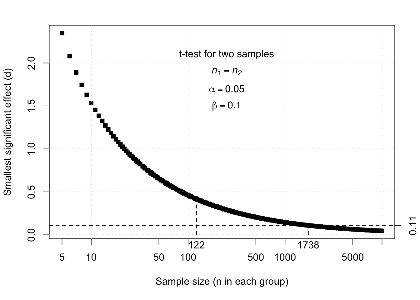
Figure 13.3: Relation between the sample size and the smallest effect (d) that is significant according to a t-test for unpaired, independent observations, with errors probabilities alpha=.05 and beta=.10.
Example 13.3: Look again at the formula (13.8) and at the Figure 13.3 which illustrate the relation between sample size and effect size. With a sample size of \(n_1=122\), we can only detect an effect of \(d=0.42\) or more, with sufficiently low probabilities of Type I and II errors again (\(\alpha=.05\), \(\beta=.10\)). To detect the very small effect of \(d=0.11\), with the same small error probabilities \(\alpha\) and \(\beta\), samples of at least 1738 girls and 1738 boys would be needed.
We can also express the effect size as the probability that the difference occurs in the predicted direction, for a randomly chosen element from the population (formulas (13.10) and (13.12)), or (if applicable) for two randomly and independently chosen elements from the two populations (formula (13.11)) (McGraw and Wong 1992). Let us again return to the grammar test from the Linguistics students (§13.2). The effect which we found is not only significant but also large. Expressed in terms of probability: the probability that a random Linguistics student achieves a score larger than \(\mu_0=73\) is 0.91. (And a randomly chosen Linguistics student thus still has 9% probability of achieving a lower score than the hypothesised population mean of 73.)
For the fictional judgements about the webpages with U or je (see Table 13.1), we find a standardised effect size of \[d = \frac{ \overline{D}-\mu_D} {s_D} = \frac{ -2.20-0 } {1.03} = -2.13\] It is then not surprising that this extremely large effect is indeed significant. We can report this as follows:
The judgements of \(N=10\) respondents about the pages with U or je as forms of address differ significantly, with on average \(-2.2\) points difference. This difference has a 95% confidence interval of \(-2.9\) to \(-1.5\) and an estimated standardised effect size \(d=-2.13\); the probability that a randomly chosen respondent judges the je-version more highly than the U-version is \(p=.98\).
13.8.1 formulas
For a single sample: \[\begin{equation} \tag{13.10} d = \frac{\overline{x}-\mu}{s} \end{equation}\] where \(s\) stands for the standard variation \(s\) of the score \(x\).
For two independent samples (see formula (13.2)): \[\begin{equation} \tag{13.11} d = \frac{ \overline{x_1}-\overline{x_2} } { s_p } \end{equation}\]
For paired observations: \[\begin{equation} \tag{13.12} d = \frac{ \overline{x_1}-\overline{x_2} } { s_D } \end{equation}\] where \(s_D\) is the standard deviation from the difference \(D\) according to the formula (13.12).
13.8.2 SPSS
In SPSS, it is usually easiest to calculate the effect size by hand.
For a simple sample (formula (13.10)), we can simply calculate the effect size from the mean and the standard deviation, taking into account the value \(\mu\) which we are testing against.
Analyze > Descriptive Statistics > Descriptives...Choose the button Options and ensure that Mean and Std.deviation are
ticked. As a result there is the required data in the output:
\(d = (84.41 - 73) / 8.392 = 1.36\), a very large effect.
For unpaired, independent observations, it is likewise the easiest to calculate the effect size by hand on the basis of the means, standard deviations, and size of the two samples, making use of the formulas (13.2) and (13.11) above.
For a single sample with two paired observations
(formula (13.12)), we can again calculate the effect
size more simply from the mean and the standard deviation of the difference.
The information is in the output of the pairwise \(t\)-test
(§13.7.3), respectively as Mean and
Std.Deviation:
\(d = -2.200 / 1.033 = 2.130\), a super large effect.
13.8.3 JASP
In JASP, the effect size can be requested when conducting the \(t\) tests, just by checking the option Effect size under “Additional Statistics”. For more detailed instructions on how to specify this using JASP, see the respective subsections for conducting a \(t\) test for a single sample (§13.2.5), a \(t\) test for two independent groups (§13.6.4), and a \(t\) test for paired observations (§13.7.4).
The output of the \(t\) test will report Cohen’s \(d\) as measure for the effect size. You can also ask for the Confidence interval of the effect size, which will typically report the 95% confidence interval of the effect size (see §13.8.5 below).
13.8.4 R
For a single sample
(formula (13.10)):
gramm2013 <- read.csv( file="data/grammaticatoets2013.csv",header=F)
dimnames(gramm2013)[[2]] <- c("score","progr")
# programs have Dutch labels, TW=Linguistics
with(gramm2013, score[progr=="TW"]) -> score.ling
# auxiliary variable
( mean(score.ling)-73 ) / sd(score.ling)
## [1] 1.359783The probability of a score larger than the population mean (the test value) 73 for a random Linguistics
student (of which we assume that \(\mu=84.4\) and \(s=8.4\)):
## [1] 0.9126321For unpaired, independent observations, we can calculate the smallest
significant effect (see also
Fig. 13.3); for which we use the function
power.t.test. (This function is
also used to construct Fig.13.3.)
With this function, you have to set the desired power as
an argument (power = \(1-\beta\); see
§14.1).
##
##      Two-sample t test power calculation
##
##               n = 122
##           delta = 0.4166921
##              sd = 1
##       sig.level = 0.05
##           power = 0.9
##     alternative = two.sided
##
## NOTE: n is number in *each* group
In the output, the smallest significant effect is indicated by delta; see also
Example 13.3 above.
For a single sample with two paired observations (formula(13.12)):
ujedata <- read.table( file="data/ujedata.csv", header=TRUE, sep=";" )
with( ujedata, mean(cond.u-cond.je) / sd(cond.u-cond.je) )
## [1] -2.13014113.8.5 Confidence interval of the effect size
Earlier, we already saw (§10.7 and §13.5) that we can estimate a characteristic or parameter of the population on the basis of a characteristic from a sample. This is how we estimated the unknown population mean \(\mu\) on the basis of the observed sample mean \(\overline{x}\). The estimation does have a certain degree of uncertainty or reliability: perhaps the unknown parameter differs in the population somewhat from the sample characteristic, which we use as an estimator, as a result of chance variations in the sample. The (un)certainty and (un)reliability is expressed as a confidence interval of the estimated characteristic. If we would repeatedly draw many samples from the same population, then the unknown population mean would be within the sample confidence interval of the mean in 95% of the resamples (see §10.7 and §13.5).
This reasoning applies not only to the mean score, or to the variance, but equally to the effect size as obtained from a single sample. After all, the effect size too is an unknown parameter from the population, which we are trying to estimate based on a limited sample. For the fictional judgements about the webpages with the formal U or informal je pronouns (see Table 13.1), we found a standardised effect size of \(d=-2.13\). This is an estimation of the unknown effect size (i.e. of the strength of the preference for the je-variant) in the population of assessors, on the basis of a sample of \(n=10\) assessors. We can also indicate the reliability of this estimation here, in the form of a confidence interval around the observed sample \(d=-2.13\).
The confidence interval of the effect size is tricky to establish though
(Nakagawa and Cuthill 2007; Chen and Peng 2015). We illustrate it here in a simple manner for
the simplest case, namely that of the \(t\)-test for a single sample,
or for two paired observations. For this, we need two elements:
firstly, the effect size expressed as a correlation (Rosenthal and Rosnow 2008, 359, formula 12.1), \[r = \sqrt{ \frac{t^2}{t^2+\textrm{df}} }\] and secondly
the standard error of the effect size \(d\) (Nakagawa and Cuthill 2007, 600,
formula 18):
\[\begin{equation}
\tag{13.13}
\textrm{se}_d = \sqrt{ \frac{2(1-r)}{n} + \frac{d^2}{2(n-1)} }
\end{equation}\]
In our earlier example of the \(n=10\) paired judgements about a webpage with U or je as forms of address we found \(d=-2.13\). We also find that \(r=.91\). With these data, we find \(\textrm{se}_d = 0.52\) via formula (13.13).
With this, we then determine the confidence interval for the effect size: \[\begin{equation} \tag{13.14} d \pm t^*_{n-1} \times \textrm{se}_d \end{equation}\] (see the correspond formula (10.12)).
After substituting \(t^*_9=2.262\) (see Appendix C) and \(\textrm{se}_d = 0.519\), we eventually find a 95% confidence interval of \((-3.30,-0.96)\). We can be 95% confident that the unknown true effect size may be within this interval (remember, if we would resample many times from the same population, then in 5% of the resamples the observed effect size would be outside this CI of the effect size). As the confidence interval is entirely below zero, we may conclude that the true effect size is probably negative, and smaller than zero. On the basis of this last consideration, we may reject H0. And: we now know not only that the preference deviates from zero, but also to what extent the (standardised) preference deviates from zero, i.e. how strong the preference for the je-version is. This new knowledge about the extent or size of the effect is often more useful and more interesting than the binary decision of whether or not there is an effect (whether or not to reject H0) (Cumming 2012).